
How to Use Statistical MAX, MIN, and MEDIAN Functions in Google Sheets
Learn how to use MAX, MIN, and MEDIAN functions in Google Sheets to enhance your data analysis and reporting capabilities.

If you work with data in Google Sheets, knowing how to use the MAX, MIN, and MEDIAN functions is a practical skill worth having. These functions help you quickly identify the highest, lowest, and middle values in your dataset, which is particularly helpful when tracking performance metrics, managing inventory, or reviewing survey responses.
This guide walks through how to use each function effectively. We'll show you how to find the highest value with MAX, the lowest with MIN, and the middle point with MEDIAN, so your analysis is both accurate and easy to follow.
Introduction to Statistical Functions
Statistical functions make it easier to analyze data in Google Sheets. Whether you're working with business reports, product stock levels, or user feedback, these tools enable you to summarize large datasets and identify patterns that matter.
Once you're comfortable using functions like MAX, MIN, and MEDIAN, you'll be able to compare values quickly, spot trends, and build clearer, more useful reports. These basics also set you up for more advanced techniques, such as calculating quartiles, identifying outliers, or examining the spread of your data.
Why Use MAX, MIN, And MEDIAN Functions?
The MAX, MIN, and MEDIAN functions help you quickly understand the spread and balance of your data.
- MAX helps you find the highest number in a set, making it ideal for identifying peak performance or maximum values without having to scan through everything manually. It’s flexible, easy to use, and works well with changing datasets.
- MIN works similarly, but finds the lowest number. It helps identify minimum thresholds, performance drops, or low points in any dataset.
- The MEDIAN gives you the middle value, which can be more useful than the average when your data has outliers or is unevenly distributed.
Breaking Down MAX, MIN, And MEDIAN Functions In Google Sheets
Let's explore the essential MAX, MIN, and MEDIAN functions to learn the syntax and see examples for each function, including MAX, MAXA, and MAXIFS; MIN, MINA, and MINIFS; and finally, the MEDIAN function.
MAX Function
The MAX function identifies the highest value in a specified range of numbers. It’s a quick way to spot the maximum value in your data. You can also use it with multiple ranges or individual numbers, which makes it flexible enough to handle different types of datasets or extra values you want to include.
Syntax of MAX Function
The syntax of the MAX function is:
=MAX(value1, [value2, ...])
Here's the break-down:
- value1, value2, ...: The arguments can be individual numbers, cell references, or ranges from which the highest value will be returned. You can include as many values or ranges as needed.
Notice, the MAX function ignores cells with text. It will only work for cells with numbers.
Example of MAX Function
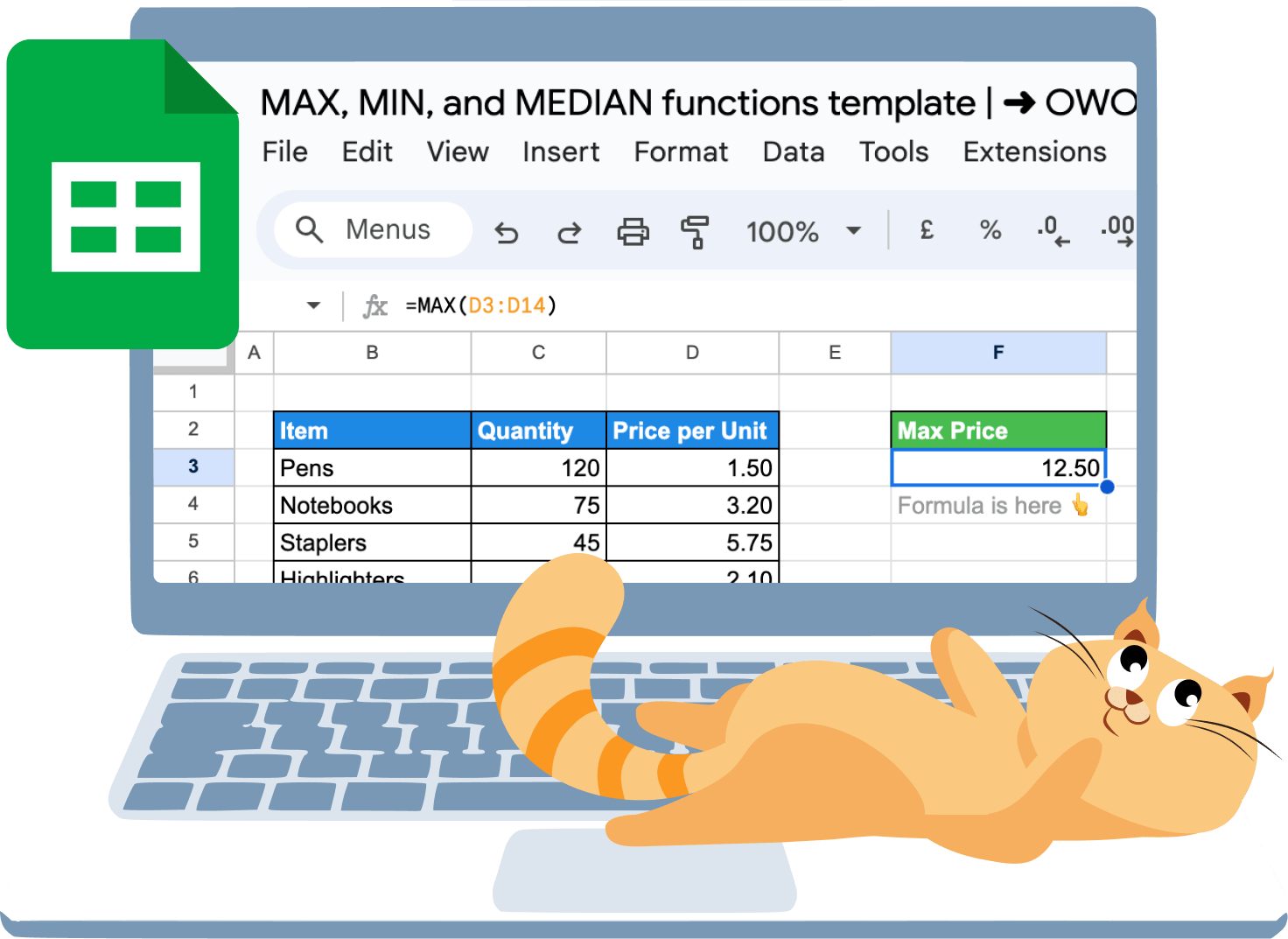
Let's say we have a list of office goods along with their quantities and prices per unit. We aim to identify the item with the highest cost per unit and display its corresponding price.
Let's apply this formula:
=MAX(D3:D14)
Here's what that means:
- D3:D14: represents the "Price per Unit" column, which contains the prices of the various office goods listed in the table.

The result of this formula indicates that calculators have the highest price per unit in this list.
MAXA Function
The MAXA function in Google Sheets is used to find the maximum value in a range, similar to the MAX function, but with a key difference.
Unlike MAX, MAXA includes logical values and text in its calculation, treating TRUE as 1, FALSE as 0, and text as zero. This makes MAXA particularly useful when your data includes a mix of numbers, logical values, and text that need to be considered in finding the maximum value.
Syntax of MAXA Function
The syntax of the MAXA function in Google Sheets is:
=MAXA(value1, [value2, ...])
Let's break it down:
- value1, value2, ...: These are the values, cell references, or ranges you want to include in the calculation.
You can include any number of arguments. The MAXA function will consider numbers, logical values (TRUE/FALSE), and text (treated as 0) in determining the maximum value.
Example of MAXA Function
Let's say we need to find out the maximum quantity of the same item in the stock, but not ignore the cells with no data, marked as N/A.
We can use this formula:
=MAXA(C3:C14)
Let's break it down:
- C3:C14: represents the "Quantity" column for the various office goods listed in the table.

The MAXA function evaluates the range C3, treating text values like "N/A" as 0. It finds the maximum value among the valid quantities, which in this case is 150.
This demonstrates how MAXA can handle mixed data types, including text, and still return the correct maximum numeric value.
MAXIFS Function
The MAXIFS function in Google Sheets returns the maximum value from a range that meets specific criteria. It allows you to filter and find the highest value based on multiple conditions.
Syntax of MAXIFS Function
The syntax of the MAXIFS function in Google Sheets is:
=MAXIFS(max_range, criteria_range1, criterion1, [criteria_range2, criterion2, ...])
Here's the breakdown:
- max_range: The range of cells from which you want to find the maximum value.
- criteria_range1: The range of cells that you want to apply the first condition to.
- criterion1: The condition or criteria to be met in the first criteria range.
- [criteria_range2, criterion2, ...]: (Optional) Additional ranges and criteria to apply. You can add multiple criteria ranges and corresponding criteria as needed.
Example of MAXIFS Function
Suppose you want to find the maximum price per unit for items where the quantity is greater than 50.
Let's use the following formula:
=MAXIFS(D3:D14, C3:C14, ">50")
Here's the explanation:
- D3:D14: This is the range where the function will find the maximum value (Price per Unit).
- C3:C14: This is the criteria range (Quantity).
- ">50": This is the criterion that the quantity must be greater than 50.

The formula will return 3.20, which is the highest price per unit for items with a quantity greater than 50 (in this case, Notebooks).
MIN Function
The MIN function is used to find the smallest value in a range of data. Whether you're tracking performance, costs, or other metrics, the MIN function provides a simple and efficient way to pinpoint the lowest value.
Syntax of MIN Function
The syntax of the MIN function in Google Sheets is:
=MIN(value1, [value2, ...])
Let's explain:
- value1, value2, ...: These are the values, cell references, or ranges from which you want to find the minimum value. You can include any number of arguments, and the MIN function will return the smallest value among them.
Example of MIN Function
Suppose you want to find the minimum price per unit among all the items listed.
For this, use the formula:
=MIN(D3:D14)
Let's break it down:
- D3:D14: represents the "Price per Unit" column, which contains the prices of the various office goods listed in the table.

The formula will return 0.05, which corresponds to the price per unit of "Paper Clips." This example illustrates how the MIN function can quickly identify the lowest value in a range, which is particularly useful for comparing costs or finding minimum thresholds in your data.
MINA Function
The MINA function in Google Sheets finds the minimum value in a range, including numbers, logical values, and text. Unlike MIN, it treats TRUE as 1, FALSE as 0, and text as 0, making it useful for datasets with mixed data types.
Syntax of MINA Function
The syntax of the MAXA function in Google Sheets is:
=MINA(value1, [value2, ...])
Let's break it down:
- value1, value2, ...: These are the values, cell references, or ranges you want to include in the calculation.
The MINA function allows for multiple arguments and takes into account numbers, logical values (TRUE/FALSE), and text (which is treated as 0) when calculating the minimum value.
Example of MINA Function
Let's say we need to check if there is no data about the quantity of items in the "Quantity" column (C3). The range includes both numeric values and text entries like "N/A", "Unknown", "No data" or "Zero".
Let's apply this formula:
=MINA(C3:C14)
Let's break it down:
- C3:C14: This is the range of quantity data.

The MINA function evaluates the range, treating text values like "N/A" or "No data" as 0. As a result, the formula returns zero as the minimum value. This indicates that some cells are not filled with quantities, and the store data needs to be updated.
MINIFS Function
The MINIFS function in Google Sheets returns the smallest value in a range that meets specified criteria. It allows you to find the lowest value based on one or more conditions.
Syntax of MINIFS Function
The syntax of the MINIFS function in Google Sheets is:
=MINIFS(min_range, criteria_range1, criterion1, [criteria_range2, criterion2, ...])
Let's break it down:
- min_range: The range of cells from which you want to find the minimum value.
- criteria_range1: The range of cells that you want to apply the first condition to.
- criterion1: The condition or criteria that must be met in the first criteria range.
- [criteria_range2, criterion2, ...]: (Optional) Additional ranges and criteria to apply. You can add multiple criteria ranges and corresponding criteria as needed.
Example of MINIFS Function
Let's say we need to find the minimum price per unit for items where the quantity is less than 50.
We can use the following formula:
=MINIFS(D3:D14, C3:C14, "<50")
Here's the explanation:
- D3:D14: This is the range where the function will find the minimum value (Price per Unit).
- C3:C14: This is the criteria range (Quantity).
- "<50": This is the criterion that the quantity must be smaller than 50.

The formula returns 3.00, which corresponds to the price per unit of "Tape Dispensers," as it is the lowest price per unit among items where the quantity is less than 50.
MEDIAN Function
The MEDIAN function is used to find the middle value in a sample set of numbers. It is a measure of central tendency, which gives you the value that lies precisely at the center of your data when it is sorted in ascending or descending order. The median divides the data set into two equal parts: the lower half, which contains values below the median, and the upper half, which includes values above the median.
Unlike the average value, the median is not affected by extreme values (outliers), making it a more accurate representation of the central value in datasets that may have skewed or uneven distributions. The MEDIAN function is handy when you need to understand the typical value in a dataset. On the other hand, if all numbers in a data set occur the same number of times, there is no mode, highlighting the absence of a most frequent value.
Syntax of the MEDIAN Function
The syntax of the MEDIAN function:
=MEDIAN(value1, [value2, ...])
Let's break it down:
- value1, value2, ...: These are the values, cell references, or ranges from which you want to calculate the median.
You can include multiple individual values or ranges, and the function will return the middle value when the numbers are sorted in order.
Example of MEDIAN Function
Suppose you want to find the median price per unit among all the items to determine the value of the stock.
Let's use the following formula:
=MEDIAN(D3:D14)
Here's the explanation:
- D3:D14: This is the range where the function will find the medium price value.

The formula returns 3.10 as the median price per unit. The median is the middle value in a sorted list of prices, distinct from the average value, which can skew.
This example also shows how the MEDIAN function helps you find the middle value in a dataset, which is especially useful when the data includes outliers or isn’t evenly distributed. It provides a more balanced view, such as a typical price per unit, so extreme values don’t skew your pricing or cost analysis.
Basic Examples Of Using MAX, MIN, And MEDIAN Functions In Google Sheets
Explore these basic examples to learn how to use the MAX, MAXA, MIN, MINA, and MEDIAN functions. Discover how they handle numbers, text, and ranges for accurate data analysis. When inputting data, you can enter data points as separate lines or separate them with commas or spaces, allowing flexibility in how you organize your entries.
Using MAX For The Largest Number With Text
When dealing with an inaccurate price list from the store that includes text entries instead of numbers, the MAX function helps you focus on what matters. It will only consider the numerical values, ignoring any text, to accurately identify the highest price.
Let's apply this formula:
=MAX(C3:C14)
The formula returns 150, which is the highest value in the "Quantity" column, disregarding cells with text values.

When dealing with a dataset that includes both numbers and text, such as an inventory list where some quantities are marked as "N/A," the MAX function proves invaluable. In this example, applying MAX to the "Quantity" column ignores the text entries and correctly sets the maximum quantity as 150.
This ensures that even with incomplete or inaccurate data, you can still extract meaningful insights and focus on the most relevant numerical information.
Using MAXA with Individual Numbers and Ranges of Cells
Suppose you want to find the maximum value in the "Quantity" column, but you also want to include additional individual values outside the table in your calculation. The MAXA function will consider these individual values, as well as any text or logical values in the table.
Let's use the following formula:
=MAXA(C3:C14, F3, 25, 35)
The formula returns 250, which is the highest value among the quantities in the table and the additional individual numbers.

The MAXA function in Google Sheets can be used to find the maximum value across both a specified range and additional individual numbers. This function considers text entries like "N/A" as 0 and evaluates all inputs, including additional cells and direct numbers, to return the correct maximum value.
Using MIN with Numbers and Text
Suppose we have a list of quantities that include both numbers and text entries, such as "N/A." We want to find the smallest numerical value in this list.
Let's use the following formula:
=MIN(C3:C14)
The formula will return 15, which is the smallest numerical value in the range.

The MIN function in Google Sheets effectively ignores text values and only considers numbers when determining the minimum value in a range.
MINA Function to Find the Smallest Value Between Two Ranges
Suppose we have two separate ranges of quantities, according to store data dispatch, that include both numbers and text entries. You want to find the smallest value across these two ranges, taking into account any text, that points to an unknown quantity of goods.
Let's apply this formula:
=MINA(C3:C8, C10:C14)
Even though the smallest numeric value in the range C10:C14 is 15, this formula returns 0. Why? Because the MINA function treats text, like the "N/A" in cell C7, as a zero, making 0 the smallest value in the combined ranges.

Unlike the MIN function, MINA includes text and logical values in its evaluation, making it suitable for datasets where such entries should be factored into the minimum value calculation.
Using the MEDIAN with Individual Cell Values and Cell Ranges
We want to calculate the median price per unit for various office supplies. The data is spread across specific cells, and we also want to include some additional individual values in the calculation.
For this, let's use:
=MEDIAN(D4,D5,D7,D10,D13)
The MEDIAN function takes these specific cells and calculates the median value.

Alternatively, to calculate the median using a continuous range of cells, we could use the following formula:
=MEDIAN(D3:D14)
This formula includes all the "Price per Unit" values from D3 to D14.

The MEDIAN function is handy in real situations where you need to identify the typical price per unit in a numeric dataset, especially when prices vary widely.
It helps ensure that outliers don't skew your analysis, providing a more accurate representation of the central price point for inventory valuation, pricing strategies, or cost analysis.
Combining Cell Values And Ranges With The MEDIAN Function
Let's assume we have a list of prices per unit for various office supplies, and we want to calculate the median value. The data includes both a range of cells and some additional individual values that are not part of the main range. The following formula could be applied:
=MEDIAN(D3:D10, F3, 7, 11)
The formula returns 4.00, which is the median of the combined data set.

The MEDIAN function can be used to calculate the median value from a combination of a range of cells and additional individual values. It's advantageous when you need to include specific outliers or additional data points in your analysis.
Advanced Applications Of MAX, MIN, And MEDIAN Functions In Google Sheets
Explore essential techniques like identifying the latest and earliest dates using MAX and MIN functions, handling negative values, and applying MAXIFS and MINIFS with multiple criteria.
Identifying The Latest Date Using The MAX Function
Suppose we have a list of office supplies with their respective supply dates. Our goal is to determine the most recent supply date from the list.
The following formula could be used:
=MAX(E3:E14)
The formula returns 14/08/2024, which is the latest date in the range.

By applying the MAX function to a range of dates, you can quickly determine the most recent entry, which is especially useful for tracking updates or recent events.
Finding The Earliest Date Using The MIN Function
Let's have a list of office supplies with their respective supply dates. So we want to determine the earliest supply date from the list.
This could be possible with the following formula:
=MIN(E3:E14)
The formula returns 05/08/2024, which is the earliest date in the range.

Applying the MIN function to a range of dates, you can quickly determine the first or oldest entry.
Using MAX and MIN Functions with Negative Values
Let's say we have a list of items with their respective discounts, all of which are negative percentages. If we want to find the discount closest to zero, which represents the least discount given, we have to apply the MAX function:
=MAX(E3:E14)
The formula returns -5%, which is the discount closest to zero in the range.

Be careful when using the MAX function with negative numbers. Because the values are negative, the number closest to zero is considered the largest.
To find the most significant discount given, which is the most negative percentage, we would apply the MIN function:
=MIN(E3:E14)
The formula returns -40%, which is the largest discount (most negative value) in the range.

The MAX and MIN functions can be used to analyze negative values in Google Sheets, making them useful for tasks like comparing discounts, losses, or other negative metrics.
Using MAXIFS with Multiple Criteria
In our list of office supplies with discounts and prices per unit, we want to find the highest price per unit for items that meet two criteria:
- The discount is less than or equal to -10%.
- The quantity available is greater than 30.
For this, let's use the formula:
=MAXIFS(D3:D14, E3:E14, "<=-10%", C3:C14, ">30")
The formula returns 5.75, which is the highest price per unit (Staplers) among items that have a discount of -10% or more and a quantity greater than 30.

The IFS suffix in MAXIFS stands for "If Statements," which means this function can evaluate multiple conditions simultaneously, enhancing your ability to perform complex data analysis with ease.
This approach is particularly useful in scenarios where you need to consider multiple factors to make well-informed decisions based on specific criteria.
💡While MAX, MIN, and MEDIAN functions help identify key statistical values, the IFS function offers a versatile approach for applying multiple conditions in a single formula. Explore our detailed guide on the IFS function to enhance your data analysis techniques in Google Sheets.

Using MINIFS with Multiple Criteria
In this example, let's find the lowest price per unit that meets specific criteria in a list of office supplies with quantities, discounts, and prices per unit. We will apply the same criteria as in the previous example:
- The discount is less than or equal to -10%.
- The quantity available is greater than 30.
For this, use this formula:
=MINIFS(D3:D14, E3:E14, "<=-10%", C3:C14, ">30")
The formula returns 0.75, which is the lowest price per unit (File Folders) among items with a discount of -10% or more and a quantity greater than 30.

In this case, the MINIFS function enabled us to filter the data by discount and quantity to find the lowest price that meets the specified criteria.
Combining MAX, MIN, And MEDIAN Functions With Other Google Sheet Functions
Learn advanced techniques by combining MAX, MIN, and MEDIAN functions with other Google Sheets functions for powerful data analysis.
Using MAX With ARRAYFORMULA
Combining the MAX function with ARRAYFORMULA in Google Sheets allows you to process a range of data efficiently, identifying the maximum value across an entire dataset. This approach is particularly useful when dealing with dynamic ranges or large datasets where you want to apply a function across multiple cells simultaneously.
Suppose we want to calculate the final price for each item after applying the discount, and then find the highest final price using the MAX function.
Let's apply this formula:
=MAX(ARRAYFORMULA(D3:D14 * (1 + E3:E14)))
Here's the breakdown:
- E3:E14: This is the range containing the discount percentages.
- 1 + E3:E14: The 1 + in this part of the formula adjusts the discounts for multiplication. Since discounts are typically expressed as negative percentages (e.g., -20%), adding 1 to these values converts them into multipliers. For example, a -20% discount becomes 1 – 0.20 = 0.80, meaning you pay 80% of the original price.
- D3:D14: This is the range containing the "Price per Unit" values.
- ARRAYFORMULA: This applies the operation across the entire range, multiplying each price by its respective discount-adjusted multiplier.
- MAX: Finally, this function returns the highest price after all discounts have been applied.
As a result, the formula identifies the highest discounted price, which in this case is $11.25 for the Calculators.

By leveraging the power of ARRAYFORMULA, we can apply the discount calculation across a range of data simultaneously, making data analysis both quicker and more efficient.
Using MIN With FILTER To Find The Smallest Non-Zero Value
You can combine the MIN and FILTER functions in Google Sheets to find the smallest value in a dataset while skipping over any zeros. This is especially helpful when zero isn’t meaningful in your analysis and you want the result to reflect only values greater than zero.
Let's adjust our regular dataset by adding a few 0 values to the 'Price per Unit' column, and then find the smallest non-zero price per unit. For this, let's apply the following formula:
=MIN(FILTER(D3:D14, D3:D14 > 0))
Let's break it down:
- D3:D14: This is the range containing the "Price per Unit" values.
- FILTER(D3:D14, D3:D14 > 0): The FILTER function filters out any prices that are not greater than zero, leaving only the non-zero values.
- MIN: Finally, the MIN function finds the smallest value among the filtered (non-zero) prices.
As a result, the price of 0.75 for Paper Clips is the smallest non-zero value.

Using FILTER with MIN allows you to exclude zero values from your data, helping you identify the smallest meaningful number and thereby improving the accuracy of your analysis.
💡 Understanding the MAX, MIN, and MEDIAN functions is crucial for statistical analysis in Google Sheets, but for more dynamic data filtering based on conditions, the FILTER function is indispensable. Explore our comprehensive guide on the FILTER function to enhance your data handling capabilities.

Using MIN with INDEX and MATCH Functions for Vertical Reverse Lookup
Combining the MIN function with INDEX and MATCH in Google Sheets allows you to perform a vertical reverse lookup, which is particularly useful when you want to find the minimum value in a column and return the corresponding value from another column.
This technique is helpful for scenarios where the relationship between data points needs to be analyzed based on the smallest value found.
Let's find the item with the lowest price per unit and return its name.
We will use this formula here:
=INDEX(B3:B14, MATCH(MIN(D3:D14), D3:D14, 0))
Here's the breakdown:
- D3:D14: This range contains the "Price per Unit" values.
- MIN(D3:D14): The MIN function identifies the smallest price in the "Price per Unit" column.
- MATCH(MIN(D3:D14), D3:D14, 0): The MATCH function finds the position (row number) of this minimum value within the D3:D14 range.
- INDEX(B3:B14, ...): Finally, the INDEX function uses the position identified by MATCH to return the corresponding item name from the B3:B14 range.
As a result, we find that Paper Clips have the lowest price of 0.05.

By leveraging MIN with INDEX and MATCH, you can efficiently perform reverse lookups, allowing you to retrieve related data based on the minimum value in a different column. This method is compelling for tasks involving relational data analysis where finding and linking minimum values is crucial.
💡 While MAX, MIN, and MEDIAN provide basic statistical insights in Google Sheets, exploring INDEX & MATCH functions can significantly enhance your data retrieval processes. Dive into our detailed guide on INDEX & MATCH to unlock more precise data extraction techniques.

Using MIN with QUERY and ARRAYFORMULA
Combining the MIN function with QUERY and ARRAYFORMULA in Google Sheets allows you to extract and analyze specific subsets of data dynamically and find the minimum value within that subset.
This approach is especially powerful when dealing with large datasets where you need to filter data based on complex criteria and then find the minimum value from the filtered results.
Suppose we want to find the minimum price per unit for items that have a quantity greater than 20, using QUERY to filter the data and ARRAYFORMULA to handle the range.
We can apply this formula:
=MIN(ARRAYFORMULA(QUERY({C3:C14, D3:D14}, "select Col2 where Col1 > 20", 0)))
Here's the breakdown:
- {C3:C14, D3:D14}: This creates an array of columns, where C3:B14 represents the "Quantity" and D3:D14 represents the "Price per Unit".
- QUERY({C3:C14, D3:D14}, "select Col2 where Col1 > 20", 0): The QUERY function selects data from the array where the quantity (Col1) is greater than 20, and returns the corresponding prices (Col2).
- ARRAYFORMULA: This function ensures that the QUERY function processes the entire array at once.
- MIN: Finally, the MIN function calculates the minimum value from the filtered results provided by the QUERY.
As a result, we have the minimum price for items with quantities greater than 20 (Paper Clips, 0.05).

This method is quite useful for handling complex data analysis tasks where you need to both filter and analyze data dynamically across large datasets.
💡 As you master statistical functions like MAX, MIN, and MEDIAN, consider advancing your data manipulation skills with the QUERY function. Check out our comprehensive guide on how to leverage QUERY for complex data queries and analyses in Google Sheets.

Using MEDIAN with IF and ARRAYFORMULA Functions
Combining the MEDIAN function with IF and ARRAYFORMULA allows you to calculate the median of a dataset based on specific conditions across an entire range without the need for manual array entry.
Suppose we want to find the median price per unit for items that have a quantity greater than 20, using ARRAYFORMULA to handle the entire range automatically, with column C as the range for Quantity.
Let's apply the formula:
=ARRAYFORMULA(MEDIAN(IF(C3:C14 > 20, D3:D14)))
Here's the breakdown:
- C3:C14: This is the range containing the "Quantity" values.
- IF(C3:C14> 20, D3:D14): The IF function checks each value in the "Quantity" column to see if it is greater than 20. If the condition is met, it includes the corresponding "Price per Unit" from the D3:D14 range in the calculation.
- ARRAYFORMULA: This function allows the IF function to process the entire range at once, applying the condition dynamically.
- MEDIAN: Finally, the MEDIAN function calculates the median of the prices that meet the condition (where the quantity is greater than 20).
The result is 2.55 which is the median price for items with quantities over 20.

This approach is particularly useful in expense reporting, where it can highlight the most representative costs for budgeting and cost control. Additionally, it aids in fair revenue recognition by calculating the median price of products that meet specific criteria.
💡 While exploring statistical functions, enhancing your conditional logic with the IF function can significantly improve data analysis. Dive into our guide on the IF function to learn how to apply conditions effectively in Google Sheets.

Using MEDIAN with FILTER Function for Conditional Filtering
Combining the MEDIAN function with the FILTER function in Google Sheets allows you to calculate the median value of a dataset based on specific conditions. This approach can be applied when you need to focus on a subset of data that meets certain criteria, ensuring that the median reflects only the relevant data points.
In this example, we’ll accomplish the same task as in the previous example but with a simpler approach, using just two functions instead of three. Here, we'll calculate the median price per unit for items where the quantity exceeds 20.
Here’s the formula:
=MEDIAN(FILTER(D3:D14, C3:C14 > 20))
Let's break it down:
- D3:D14: This is the range containing the "Price per Unit" values.
- FILTER(D3:D14, C3:C14 > 20): The FILTER function filters the "Price per Unit" values based on the condition that the corresponding "Quantity" values in C3:C14 are greater than 20.
- MEDIAN: Finally, the MEDIAN function calculates the median of the prices that meet the condition (where the quantity is greater than 20).
The formula returns the same value of 2.55 which is the median price for items with quantities greater than 20.

This method is particularly effective in scenarios where conditional filtering is needed to derive meaningful insights from your data.
Addressing Common Challenges with MAX, MIN, and Other Related Functions
Explore solutions for common challenges when using MAX, MIN, and related functions, including issues with non-numeric values, incorrect range references, division by zero, and various error messages like #VALUE!, #N/A, and #ERROR!
Non-Numeric Values Errors While Using MAX function
⚠️ Error: The MAX function is designed to work with numbers, so if text or other non-numeric values are included in the range, they may be ignored, or the function may return an error, leading to inaccurate outcomes.
To avoid this, ensure that the range contains only numeric data or use additional functions like FILTER to exclude non-numeric values.
Incorrect Range References in the MAX and MIN Functions
⚠️ Error: Incorrect range references can lead to inaccurate results or errors. If the selected range is too large, too small, or doesn't include the intended data, the function might return an incorrect value or fail to work properly.
Always double-check that your range references accurately reflect the data you want to analyze to avoid these issues.
Division by Zero Error while Using MIN
⚠️ Error: A division by zero error in the MIN function occurs when the formula attempts to divide by zero, which is mathematically undefined. This typically happens when the range includes a cell with a zero value used in a division operation.
✅ Solution: To avoid this, ensure that your data does not include zero in divisions or use error-handling functions like IFERROR to manage such cases.
#VALUE! Error Due to Unequal Range Sizes in MAXIFS
⚠️ Error: A #VALUE! error in the MAXIFS function is often caused by unequal range sizes. When the criteria range and the data range are not the same size, the function cannot process the data correctly and returns an error.
✅ Solution: To fix this, ensure that all ranges used in the MAXIFS function are of equal size and correctly aligned with each other.
Incorrect Results in MINA Due to Empty Cells Treated as Zero
⚠️ Error: The MINA function may return incorrect results if there are empty cells in the range, as these cells are treated as zero. This can skew the minimum value calculation, especially when zeros are not expected.
✅ Solution: To avoid this, either ensure that all cells contain valid data or use a different function like MIN to exclude empty cells from the calculation.
#N/A Error with MINIFS Function
⚠️ Error: A #N/A error in the MINIFS function occurs when no data matches the criteria specified. This happens when the function cannot find any values that meet the given conditions, leading it to return #N/A.
✅ Solution: To prevent this, verify that your criteria are accurate and that the dataset includes values that meet these criteria.
#ERROR! While using MAXA
⚠️ Error: A #ERROR! message in the MAXA function often arises when non-numeric data, such as text or error values, is included in the range. MAXA can handle non-numeric data, but if the data cannot be interpreted as a number, it may produce an error.
✅ Solution: To resolve this, clean your data to ensure that only valid numeric values are included in the range.
Best Practices and Tips for Using MAX, MIN, and MEDIAN Functions
Implementing best practices with MAX, MIN, and MEDIAN functions ensures accurate and efficient data analysis. Follow these tips to optimize your use of these functions, especially when working with large datasets or complex calculations.
Filter Your Data While Using Large Datasets for MAX Function
When working with large datasets, filtering your data before applying the MAX function helps ensure you’re analyzing the most relevant values. This approach not only speeds up calculations but also prevents errors by excluding non-relevant data points.
Using filters allows you to focus on specific criteria, such as dates, categories, or other conditions, making your analysis more precise and meaningful.
Use Named Ranges for MAX Function
Named ranges for the MAX Function make it easier to reference specific datasets and reduce the chance of errors caused by selecting incorrect ranges.
This practice is particularly helpful when working with complex spreadsheets, as it simplifies formula creation and makes your calculations more transparent and easier to audit.
Use Cell References in MIN Function for Dynamic and Flexible Formulas
Incorporating cell references in the MIN function creates dynamic and flexible formulas that can adapt to changes in your data. By referencing cells rather than hard-coding values, your formulas will automatically update when data changes, ensuring accuracy without the need for manual adjustments.
This approach is particularly beneficial in scenarios where data is frequently updated or modified.
Ensure Values Are Numeric to Prevent Errors while Using MIN
To prevent errors when using the MIN function, always ensure that the values within your selected range are numeric. Non-numeric values, such as text or blank cells, can cause the function to return incorrect results or errors.
Before applying the MIN function, clean your dataset to remove or correct any non-numeric entries, ensuring a smooth and accurate calculation.
Sort Your Data in Ascending Order Before Applying the MEDIAN Function
Sorting your data in ascending order before applying the MEDIAN function can improve the clarity of your results, especially in large datasets. Although the MEDIAN function does not require sorted data, ordering your data beforehand can make it easier to understand and verify the results. This practice is particularly useful when visually inspecting or presenting your dataset.
Combine the QUARTILE Function with MEDIAN for Deeper Data Distribution Insights
Combining the QUARTILE function with MEDIAN provides a more comprehensive analysis of your data distribution. While the MEDIAN gives you the central value, the QUARTILE allows you to examine the spread of your data by dividing it into four parts.
This combination helps identify patterns and outliers, offering deeper insights into the distribution and variability of your dataset.
Key Google Sheets Formulas for Advanced Data Analysis
Google Sheets provides powerful formulas that can significantly improve your data analysis. These essential functions allow you to efficiently manage, analyze, and interpret complex data with greater precision and ease.
- VLOOKUP: VLOOKUP allows you to search for a specific value in one column and return a corresponding value from another column in the same row. It’s commonly used for vertical lookups in large datasets.
- UNIQUE: The UNIQUE function returns unique values from a range, eliminating duplicates and helping streamline data for analysis or reporting.
- COUNTIF: COUNTIF counts the number of cells that meet a specific condition within a range. It’s useful for filtering data based on criteria.
- IMPORTRANGE: This function enables you to import a range of data from one Google Sheets file to another, making it ideal for combining data from multiple sources.
- GOOGLEFINANCE: GOOGLEFINANCE retrieves real-time financial data, such as stock prices, currency exchange rates, and other market trends, directly into Google Sheets.
- AVERAGE: The AVERAGE function calculates the mean of a set of numbers, helping you quickly find the central value in a dataset. It’s useful for analyzing trends and making comparisons across different data points.
- SUM: The SUM function adds up a range of numbers, making it one of the most basic and frequently used functions for calculating totals in datasets.
Visualize Your Data with OWOX: Reports, Charts & Pivots Extension
Easily create dynamic pivots and visualize data by integrating BigQuery with Google Sheets using the OWOX: Reports, Charts & Pivots Extension. Simplify data management, automate imports, and gain powerful insights for informed decision-making!
Frequently asked questions


Finally, a tool that doesn't ask business users to learn a new dashboarding UI. Our marketing team already knows Sheets. OWOX just delivers the right data.
Joinable data marts concept was the thing that sold us. We can now use the semantic layer without building one.
Self-hosted the OSS version on Digital Ocean. Zero vendor lock-in. Contributed a Shopify connector back in week two.