How to Use Google Sheets IF for Conditional Logic

Want your spreadsheets to work smarter? The IF function in Google Sheets helps you apply simple logic to your data, so you can automate decisions and cut down on manual effort. Whether you're tracking tasks, reviewing reports, or running a campaign, it makes everyday work faster and easier.

From monitoring project progress to forecasting sales or evaluating campaign success, the IF function supports a range of everyday tasks. In this article, we’ll show you how to use the IF function effectively in Google Sheets, covering syntax, use cases, examples, and tips for combining it with other functions

Understanding the Basics of the IF Function

The IF statement in Google Sheets checks whether a condition is true or false and gives a result based on that. It’s useful when you want your sheet to make decisions automatically, like showing “Yes” if a target is met. This makes it easier to manage data, build dashboards, and create smarter spreadsheets.

The IF function makes it possible to automate calculations, categorize data based on specific criteria, and fill cells automatically depending on the conditions you set.

Join us as we explore the fundamentals of the IF function, equipping you to enhance your reports and simplify complex tasks.

IF Function Syntax

The IF function in Google Sheets lets you set up logic that runs only when a certain condition is met. It’s a simple yet powerful way to make your spreadsheets more dynamic, returning different results depending on whether the condition is true or false.

Here’s the syntax:

=IF(logical_expression, value_if_true, value_if_false)

Let's break down what these parameters represent:

• logical_expression: a logical expression that Google Sheets evaluates. It must return either TRUE or FALSE.
• value_if_true: the value or action the function returns or executes if the condition is TRUE. It can be a number, text, cell reference, or even another formula.
• value_if_false: the value or action the function returns or executes if the condition is FALSE. Similar to the value_if_true, it can be varied in type, including numbers, text, or other formulas.

A complete formula requires all three arguments and must end with a closing parenthesis to ensure it works correctly. For example: =IF(A1>10, "High", "Low") is a complete formula.

Note: When specifying text values in your formula, always enclose them in quotation marks to avoid syntax errors and ensure the formula functions properly. Watch out for misplaced commas, parentheses, or missing quotes—they’re common IF function errors.

Example of IF Function

When you understand how the IF function works, you can make your spreadsheets react to different situations and handle repetitive decisions automatically.

Here’s a simple example to show how it works. If you’re using text values like “Pass” or “Fail” in your formula, make sure to put them in double quotes so the formula runs correctly.

Let’s take a look at an example of the IF function:

=IF(B2 >= 50, "Pass", "Fail")

Here:

• B2 >= 50: The value in B2 is greater than or equal to 50.
• "Pass": If B2 is 50 or greater, the formula will return "Pass".‍
• "Fail": If B2 is less than 50, the formula will return "Fail".

Leverage the IF Function in Google Sheets!

By using this function, you can dynamically control the output of your data, automate tasks, and streamline your reporting processes with simple yet powerful logic statements.

Get your free template now!

Practical Applications of IF Function (With Examples)

The IF formula in Google Sheets is a powerful tool for transforming data management and reporting. This chapter explores real-world applications, showing how to use it for tasks like managing inventory, tracking project milestones, analyzing financial data. You can also use the IF function to analyze sales data for reporting and performance evaluation.

These examples will demonstrate how to make your data work smarter. If you’re ready to take your analysis further, try connecting Google Sheets to BigQuery. It’s easy to set up, and our guide walks you through every step.

Using the IF Function and Numerical Values

You can use numbers in the IF function’s arguments just as easily as text, allowing for flexible decision-making in your spreadsheets. This function enables not just filling cells with specific values based on conditions, but also performing calculations and returning the corresponding value for each condition.

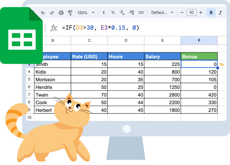
Let’s say you have a list of employees with their weekly working hours, hourly rates, and salaries, and you want to reward employees who work over 30 hours a week with a bonus. Let’s see how you can use the IF function to automate this.

Enter the following formula in cell F3:

=IF(D3>30, E3*0.15, 0)

This setup calculates a 15% bonus of the weekly salary for those who work more than 30 hours a week. Drag this formula down the column to apply it across all employees.

Using the IF Function to Work with Blanks / Non-blanks

The IF function in Google Sheets can handle both blank and non-blank cells, effectively using a logical expression. By specifying conditions based on whether cells contain data or are empty (“”), you can automate decisions. 

Let’s consider some employees who haven’t yet applied their working hours. In such cases, we need to mark their salary cells with “No data.”

To automate this, we apply the following formula in cell E3:

=IF(D3="", "No Data", C3*D3)

Dragging this formula down will apply it to all employees. This will allow you to spot employees who didn’t provide their working hours at a glance.

Tip: Alternatively, you can use the ISBLANK function for formula checks to identify empty cells. Formula checks for blank cells can use either ISBLANK or standard comparison operators like ="" or <>"" within IF statements. For example, you could write =IF(ISBLANK(D3), "No Data", C3*D3) or use a standard comparison operator like =IF(D3<>"", C3*D3, "No Data") to achieve similar results.

Using the IF Function with Text

You can also employ the IF function to generate a specific value from cells containing an exact text string. When using text values as arguments in the IF function, always enclose the text values in double-quotes (e.g., "No Data") to ensure the formula works correctly. This feature lets you set up different outcomes based on specific text values in your data, using multiple conditions in one formula.

Let’s consider some employees who still need to report their working hours. It’s important to note that no bonus will be awarded until they submit their data. 

In this formula, if the text value in E3 is "No Data", the value returned is "No Bonus". Otherwise, the value returned is the result of E3 multiplied by 0.15.

Let’s apply the formula in cell F3:

=IF(E3="No Data", "No Bonus", E3*0.15)

As soon as you drag the formula down, it will be applied to all the employees.

Pro Tip: Using the ARRAYFORMULA function in this use case allows you to apply a formula to an entire column, processing each cell according to the specified conditions. This can simplify your calculations, avoiding copying formulas or dragging them down across multiple rows manually.

To make the same calculation using the IF with ARRAYFORMULA function, here is the formula you should apply:

=ARRAYFORMULA(IF(E3:E9="No Data", "No Bonus", E3:E*0.15))

Again, ensure that text values like "No Data" and "No Bonus" are enclosed in double-quotes. The values returned by this formula will be "No Bonus" for employees with missing data, or their calculated bonus for those who have reported hours.

Using ARRAYFORMULA simplifies the process and ensures that your spreadsheet remains dynamic and easy to update.

• less than 30 hours: Label as “Low”
• 30 to 40 hours: Label as “Regular”
• over 40 hours: Label as “High”

In this nested IF formula, the value returned will be "Low" if D3 is less than 30, "Regular" if D3 is between 30 and 40, and "High" if D3 is over 40.

Let’s apply the engagement level formula in cell G3:

=IF(D3<30,"Low",IF(D3<=40, "Regular",IF(D3>40, "High")))

Then, by dragging it down, we can apply it to the entire list of employees, efficiently categorizing workers based on their weekly hours.

Using IF Function (Equal To) for Conditional Logic

The IF function in Google Sheets is highly versatile and can be used to perform conditional logic based on whether a value is equal to a specified criterion. It evaluates a logical test that returns a boolean result, either TRUE or FALSE, and then performs an action if the condition is met. 

These IF statements are particularly useful when you need to evaluate data and return results or actions depending on exact matches. 

For instance, if you need to find out which workers didn’t get paid because they didn’t submit their working hours’ data, you can flag these cases by setting the parameter “No data” in their ‘Salary’ cell:

=IF(E3="No Data", "Not paid", "Paid")

Then you can incorporate this formula into the full list of employees by dragging the formula down.

Using the IF Function (Greater Than) for Conditional Logic

One common usage of the IF function is checking if a value is greater than a specified threshold. This comes in handy for things like performance reviews, financial checks, or managing inventory, any situation where decisions depend on numbers. You can use comparison operators like >, <, >=, and <= in your IF formulas to check if certain conditions are met. For example, if you want to pay a bonus to all employees who worked more than 30 hours per week, you can set “>30” as the condition.

Then, in the “Bonus” column, you can determine if they qualify for the bonus based on this condition:

=IF(D3>30,"Bonus", "No Bonus")

While mastering the IF function enables you to make logical decisions within your data, pairing it with VLOOKUP can significantly expand your data-handling capabilities. Explore our guide to learn how to effectively use VLOOKUP with the IF function for more advanced data manipulation.

Combining the IF Function with Other Google Sheets Functions

Combining the IF function with other functions in Google Sheets unlocks powerful capabilities for data manipulation and analysis. Combining IF with functions like AND or OR lets you evaluate multiple conditions and perform more advanced data analysis.

You can also integrate IF with functions like VLOOKUP, SUM, ISNUMBER, and ISTEXT to build dynamic formulas that automate tasks and adapt to various data inputs, enhancing your spreadsheet’s flexibility and efficiency.

Using IF with Logical Operators

Using the IF function with AND, OR, or NOT in Google Sheets helps you handle more detailed logic. These operators let you test several conditions at once, making it easier to handle situations where your formula needs to follow more than one rule.

It also helps determine if all or at least one condition is met, enhancing the flexibility and power of your IF statements in real-world scenarios.

Applying IF with the AND function

Combining the IF function with the AND function allows you to evaluate multiple conditions simultaneously. The Google Sheets IF-THEN formula, synonymous with the IF function, executes an action based on a condition.

The AND function returns TRUE only if all given conditions are met; otherwise, it returns FALSE. Using these together, you can create formulas that depend on multiple criteria being true. 

Let’s say you want to provide a bonus to motivate workers who have a low hourly rate but work more than 30 hours per week. To define these criteria in a formula using Google Sheets, you can combine two logical conditions:

• The hourly rate is less than or equal to $20.
• Weekly working hours are more than 30.

These conditions can be reflected in the formula:

=IF(AND(C3<=20, D3>30),"Bonus", "No Bonus")

Using the IF function in combination with the AND function lets you check both conditions (hourly rate and working hours) simultaneously. 

Note: In more complex scenarios, you can use nested IFs with AND to evaluate multiple conditions and handle different outcomes based on various criteria.

Utilizing IF with OR function

When you combine the IF function with OR in Google Sheets, you can check several conditions at once and return a result if any of them are true. This is especially useful when different scenarios can lead to the same outcome, making your formulas more flexible and efficient.

The OR function checks multiple conditions and returns TRUE if at least one of them is true. It returns FALSE only if all conditions are false. 

Let’s say you want to motivate workers by providing a bonus to those who either have a low hourly rate or those who work more than 30 hours per week. This means you can define a bonus even if only one of these criteria is met.

For this situation, you can use the following formula:

=IF(OR(C3<=20, D3>30),"Bonus", "No Bonus")

Tip: You can also use OR to check if a value matches multiple options, or if a date falls within more than one range. For handling many conditions, consider multiple IFs or the SWITCH function for cleaner, more efficient formulas.

The combination of IF with OR is especially useful when decisions are based on a variety of possible outcomes.

Using IF with AND & OR conditions

Combining the IF function with both AND and OR functions in Google Sheets allows you to build complex conditional logic that evaluates multiple criteria with precision. Utilizing statements in Google Sheets, such as nested IF statements, enables you to perform intricate logical evaluations and compare the functionality of traditional IF statements with IFS for different use cases. 

The IFS function in Google Sheets is a simpler alternative to using multiple nested IF statements. It lets you test several conditions in one formula, making your logic easier to read and manage. This helps keep your formulas clean, especially when you’re dealing with lots of different conditions.

The IFS function syntax is easier to read compared to nested IF statements due to less complexity, making it a preferred choice for handling multiple conditions in a straightforward manner.

Imagine you are managing a bonus system for employees and want to award bonuses based on the following criteria:

• Low hourly rate: The employee earns less than $20 per hour.
• High weekly hours: The employee works more than 30 hours per week.
• Low income: If the weekly salary is below $1,000.

Let’s reflect it all in a formula:

=IF(OR(AND(D3<20, C3>30), OR(E3<1000)), "Bonus", "No Bonus")

Using the IF function combined with AND and OR conditions in Google Sheets allows you to create robust formulas that can handle intricate decision-making scenarios. This is especially helpful when you need to automate decisions based on several conditions. It makes managing and analyzing your data easier, faster, and more reliable.

Applying IF with DATE Functions

Applying the IF function with DATE functions in Google Sheets enables you to perform conditional checks based on dates by understanding the Google Sheets syntax. You can compare dates, check if a date is in the past or future, or calculate age.

For instance, you want to give a bonus to all employees who have been with the company since before 2024. By checking their contract date and comparing it with the beginning of the year, you can identify employees who started their contracts before 2024.

Let's add it to the formula:

=IF(D3<DATE(2024, 1, 1), "Bonus", "No Bonus")

Combining logical operators with date functions, you can extend the capabilities of your data operations to include calendar-based calculations.

Using IF with ISNUMBER, ISTEXT Functions

Using the IF function with ISNUMBER and ISTEXT functions in Google Sheets allows for precise data validation and conditional logic based on cell content types.

For example, you need to find out if the employee has a weekly salary or if their salary is not applied due to a lack of working data. If the salary is not calculated, it means it has not been paid yet.

Let's use this formula:

=IF(ISTEXT(E3),"Not paid",IF(ISNUMBER(E3),"Paid"))

Here's the formula breakdown:

• (ISTEXT(E3)): This checks if E3 contains text (non-numeric), such as "No Data". If true, the formula returns "Not paid".
• (ISNUMBER(E3)): If the first check is false (i.e., the cell does not contain text), it checks whether the cell contains a number. If this is true, it returns "Paid".

This formula helps effectively categorize employees' payment status based on the presence of either textual descriptions or numerical salary data. This is particularly useful in managing payroll data where quick visual identification of payment status is needed, ensuring clarity and efficiency in financial documentation and analysis.

Using IF with SUM Function

Google Sheets provides powerful tools for dynamic data analysis, one of which involves combining the IF and SUM functions to execute conditional sums based on your specified criteria using logical expressions. This capability is especially useful when you need to aggregate data that meets certain conditions.

For example, let's say you need to calculate the total working hours for employees who started working at your company before the year 2024. To do this, you'll utilize a formula that integrates SUM, ARRAYFORMULA, IF, and DATE functions to selectively add up hours only for those employees who meet the date criteria.

Let's see how this formula looks:

=SUM(ARRAYFORMULA(IF(E3:E9 < DATE(2024, 1, 1), D3:D9, 0)))

• ARRAYFORMULA: It allows the IF function to be applied to each element of the array (each row in your range).
• IF(E3:E9 < DATE(2024, 1, 1), D3:D9, 0): This part checks each date in the range E3:E9. If the date is before January 1, 2024, it selects the corresponding hours from D3:D9; otherwise, it returns 0.
• SUM(...): It sums up all the values that meet the condition returned by the ARRAYFORMULA

By applying this formula, you can calculate the total hours for employees who started their roles before 2024, ensuring your analysis is both accurate and efficient.

Using IF with COUNT Function

Using the IF function with the COUNT function in Google Sheets enables you to count cells that meet specific criteria.

In Google Sheets, the combination of the IF function with the COUNT function allows for conditionally counting cells based on specific criteria, enabling you to make decisions based on these counts.

Let’s say you want to track how many employees failed to submit their working hours in a given week.

The formula used is:

=IF(COUNT(D3:D9) > 5, "More than five employees", "Five or fewer employees")

This formula counts all the cells from D3 to D9. If the count is greater than 5, it returns "More than five employees." Otherwise, it returns "Five or fewer employees."

Key Notes:

• This approach is particularly useful in scenarios where you need to apply a simple count across a range and derive a binary outcome based on that count.
• It's essential to ensure that your data range (D3:D9 in this example) accurately reflects the cells you intend to count to avoid errors in your logic.

By using the IF function together with COUNT, you can easily monitor and react to data patterns directly within your spreadsheet. This method is straightforward and effective for routine checks that influence workflow decisions or summaries.

Best Practices for Using Conditional Logic in Google Sheets

This section covers best practices for using conditional logic in Google Sheets, including optimizing reporting and analysis with the IF function. Using a formula builder can simplify the creation of complex IF statements, helping you build accurate logic faster. Learn to set clear conditions and combine functions for more advanced scenarios to enhance your spreadsheet skills.

Plan Your Logic

When using conditional logic in Google Sheets, start by knowing what you want your formula to do and what conditions it should check. Map out the logic clearly, and choose functions like IF, AND, or OR based on your needs. Always test your formula on a small sample of data to make sure it gives the right results. If the IF function is not returning the expected results, check that the logical expression is correctly formatted, as errors in the logical test can lead to incorrect outputs.

Simplify Complex Formulas

Simplify complex formulas in Google Sheets by breaking them into smaller steps or using helper columns. Use named ranges to clarify references, and employ ARRAYFORMULA to handle repetitive calculations efficiently. Document your logic with comments to make your formulas more readable and maintainable.

Use Named Ranges

Named ranges in Google Sheets make formulas easier to read and manage by replacing cell references with descriptive names. For example, if you have a range of cells for employee hours A1:A10, you can name it EmployeeHours. Then, instead of =SUM(A1:A10), you use =SUM(EmployeeHours). This improves clarity, reduces errors, and is especially helpful when working with complex logic or large datasets.

Validate Formulas

To validate formulas in Google Sheets, check for errors using built-in tools, and test with various data samples to ensure accuracy. Document any changes and their effects using an audit trail. Seek peer reviews for fresh insights, and compare results with expected outcomes to confirm correctness.

Troubleshooting Common Challenges With the IF Function

The IF function can sometimes return errors or give unexpected results. Knowing how it works makes it easier to spot issues, like mistakes in your logic, data type mismatches, or problems with nested IFs. Troubleshooting these early can save you time and help you keep your spreadsheets accurate and running smoothly.

Handling #DIV/0! Error

⚠️ Error: The #DIV/0! error occurs in Google Sheets when attempting to divide a number by zero or an empty cell, which is mathematically undefined.

✅ Solution: To address #DIV/0! errors, use the IF function to check for zero denominators before division. Alternatively, employ IFERROR to replace errors with custom messages or default values. Regularly validate data to avoid empty cells or zeros in division formulas—this helps keep your results accurate.

Resolving #VALUE! Error

⚠️ Error: The #VALUE! error occurs due to incompatible data types or incorrect function arguments.

✅ Solution: Ensure all operands are of compatible types and correct any data type mismatches. Use functions like IFERROR to handle errors gracefully by providing alternative outputs or error messages.

Fixing #REF! Error

⚠️ Error: The #REF! error in Google Sheets indicates invalid cell references, often due to deleted or moved cells referenced in formulas.

✅ Solution: Review and update formulas to reference valid cell ranges. Ensure cells or ranges are not deleted or relocated inadvertently to prevent these errors.

Addressing #N/A Error with IFNA

⚠️ Error: The #N/A error often arises when a function like VLOOKUP or MATCH cannot find the required value in the specified range, disrupting data analysis and calculations.

✅ Solution: The IFNA function can be combined with the IF function to handle #N/A errors gracefully. Using IFNA lets you show a custom value or message instead of an #N/A error, making your data easier to read and work with.

Correcting #NAME? Errors

⚠️ Error: The #NAME? error occurs when the formula references an unrecognized function name or misspelled function.

✅ Solution: Verify the function names are spelled correctly and supported by Google Sheets. Make sure your formulas are written correctly and reference the right cells to avoid errors.

Searching through large datasets to find specific information can be overwhelming—especially if you're not a data expert.

However, advancements in technology have led to the development of specialized tools that streamline this process, allowing users to navigate through vast amounts of data with ease.

Enhance Your Data Analysis with Advanced Google Sheets Formulas

Google Sheets provides a wide range of powerful formulas that help streamline data analysis and automate tasks across your spreadsheets.

• Pivot Tables: Streamlines data summarization and analysis, enabling quick identification of patterns and trends through automated data organization.
• QUERY: Lets you use a SQL-like language to handle complex tasks in your spreadsheet—like filtering, sorting, and summarizing data—all in one formula.
• CONCATENATE: Merges multiple text segments into a single string, making it easier to amalgamate text from various cells.
• UNIQUE: Eliminates duplicate entries from a specified data range, ensuring only unique values are displayed.
• MATCH Function: Searches for a specific item within a range and returns its relative position, optimizing value location and data organization.
• FILTER Function: Filters and displays data that meets specified criteria, ideal for focusing analyses on pertinent data subsets.

Empower Your Data Analysis with OWOX: Reports, Charts & Pivots Extension

With the OWOX: Reports, Charts & Pivots Extension add-on, you can seamlessly import BigQuery data into Google Sheets and turn raw data into actionable insights in just a few clicks. Build dynamic reports, pivot tables, and charts to monitor key metrics and track performance effortlessly.

The intuitive interface lets you filter and customize your data with ease, ensuring you focus only on what matters. Equip yourself with the tools you need for smarter analysis and better decision-making, right inside Google Sheets.

‍