VLOOKUP in Google Sheets: formula, VLOOKUP from another sheet, and examples
VLOOKUP finds a value in the first column of a range and returns a value from the same row of another column. This guide covers the formula, VLOOKUP from another sheet and from another spreadsheet, partial matches, comparing lists, several columns at once, and the errors the function returns.

VLOOKUP looks for a value in the first column of a range and returns the value from the same row of another column:
=VLOOKUP(F3, $B$3:$C$10, 2, FALSE)
The formula finds the name in F3 in column B and returns the salary from column C.
| You need | Formula |
|---|---|
| VLOOKUP from another sheet (tab) | =VLOOKUP(B4, Employees!$B$4:$D$11, 3, FALSE) |
| VLOOKUP from another spreadsheet | =VLOOKUP(B2, IMPORTRANGE("spreadsheet_url", "Employees!B4:D11"), 3, FALSE) |
| A match on the beginning of the text | =VLOOKUP(F2 & "*", B3:C10, 2, FALSE) |
| Your own text instead of #N/A | =IFNA(VLOOKUP(F3, B3:D10, 3, FALSE), "Not found") |
| Several columns at once | =ARRAYFORMULA(VLOOKUP(G4:G6, B3:E10, {2, 3, 4}, FALSE)) |
VLOOKUP syntax
=VLOOKUP(search_key, range, index, [is_sorted])
- search_key: the value to look for.
- range: the table to search. VLOOKUP looks for the key in the first column of this range only.
- index: the number of the column to return, counted from the left edge of the range. The first column is 1.
- is_sorted (optional): FALSE (or 0) for an exact match. TRUE, or nothing, tells VLOOKUP that the first column is sorted and that the nearest match is good enough.
Always write FALSE unless you are deliberately looking up ranges such as price tiers. Without it, a key that is not in the table does not return an error: VLOOKUP returns the value of some other row.
Example of VLOOKUP
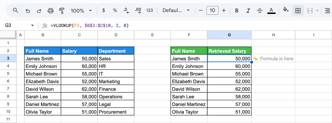
The table holds names in column B, salaries in column C and departments in column D. A second table lists some of the names, and the salary of each has to be pulled in next to it:
=VLOOKUP(F3, $B$3:$C$10, 2, 0)
- F3: the name to look for.
- $B$3:$C$10: the range to search. The names are in its first column, the salaries in its second. The dollar signs keep the range in place when the formula is copied down.
- 2: return the second column of the range, the salary.
- 0: the same as FALSE, an exact match.
Exact and partial matches
Exact match
To find the department of an employee by email address:
=VLOOKUP(G2, B3:D10, 3, FALSE)
- G2: the email address to look for.
- B3:D10: the range, with the email addresses in its first column.
- 3: the third column of the range, the department.
- FALSE: exact match. If the address is not in column B, the result is #N/A.
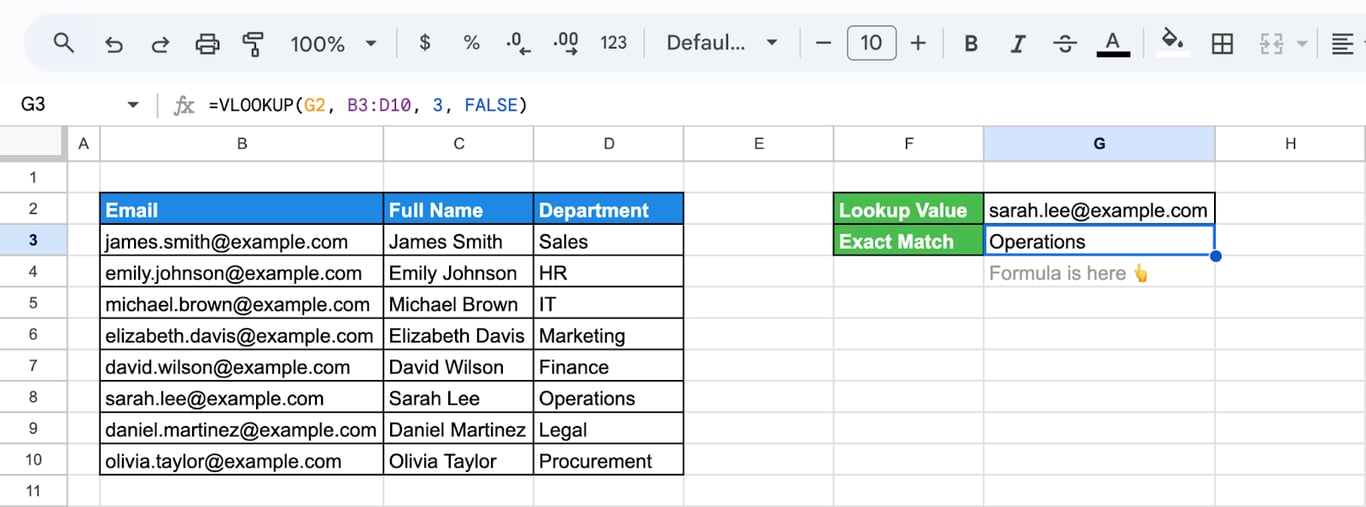
The comparison ignores case: “SARAH.LEE@example.com” finds the same row.
Partial match with a wildcard
With FALSE as the last argument, VLOOKUP accepts wildcards in the key. An asterisk stands for any number of characters, a question mark for one. To find a row by the beginning of a name:
=VLOOKUP(F2 & "*", B3:C10, 2, FALSE)
- F2 & “*”: the text typed in F2 followed by anything, for example “eli*”.
- B3:C10: names in the first column, email addresses in the second.
- 2: return the email address.
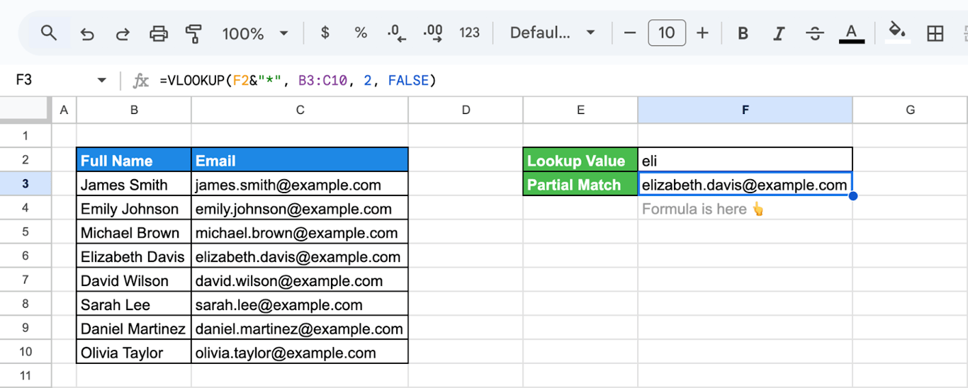
With “eli” in F2 the formula returns the email of Elizabeth Davis. If several names start with the same letters, VLOOKUP returns the first one in the table. Use "*" & F2 & "*" to match the text anywhere in the cell.
OWOX Data Marts
See your first report built in real time. 15 minutes.
- Connect your data warehouse
- Pick your metrics
- Get a live Google Sheets report
In the time it takes to write a ticket. Then imagine never writing that ticket again.
Book a DemoWe'll use your actual use case
Compare two lists
VLOOKUP can check which values of one list also appear in another. Look up each value of the first list in the second one and return the first column:
=VLOOKUP(C3, D$3:D$10, 1, FALSE)
- C3: an email from the left list.
- D$3:D$10: the right list, locked with dollar signs.
- 1: return the found value itself.
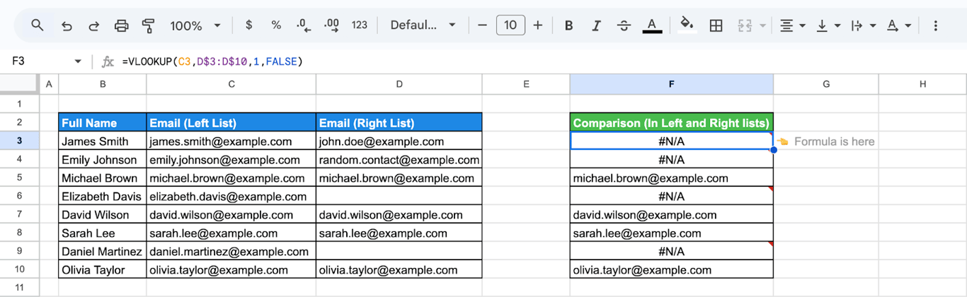
Addresses that are in both lists are returned; the ones missing from the right list show #N/A. For a clean yes or no, wrap the formula: =IF(ISNA(VLOOKUP(C3, D$3:D$10, 1, FALSE)), "Missing", "Found").
VLOOKUP with multiple criteria
VLOOKUP with multiple criteria
VLOOKUP takes one key. To look up by two values, such as first name and last name, join them into one. First add a helper column to the table that joins the two columns:
=C3&D3
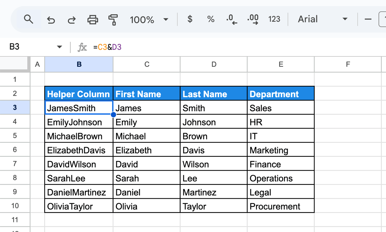
Then join the two search values in the same way and look them up in the helper column:
=VLOOKUP(H2&H3, B3:E10, 4, FALSE)
- H2&H3: first name and last name joined, “JamesSmith”.
- B3:E10: the range, with the helper column first.
- 4: the fourth column, the department.
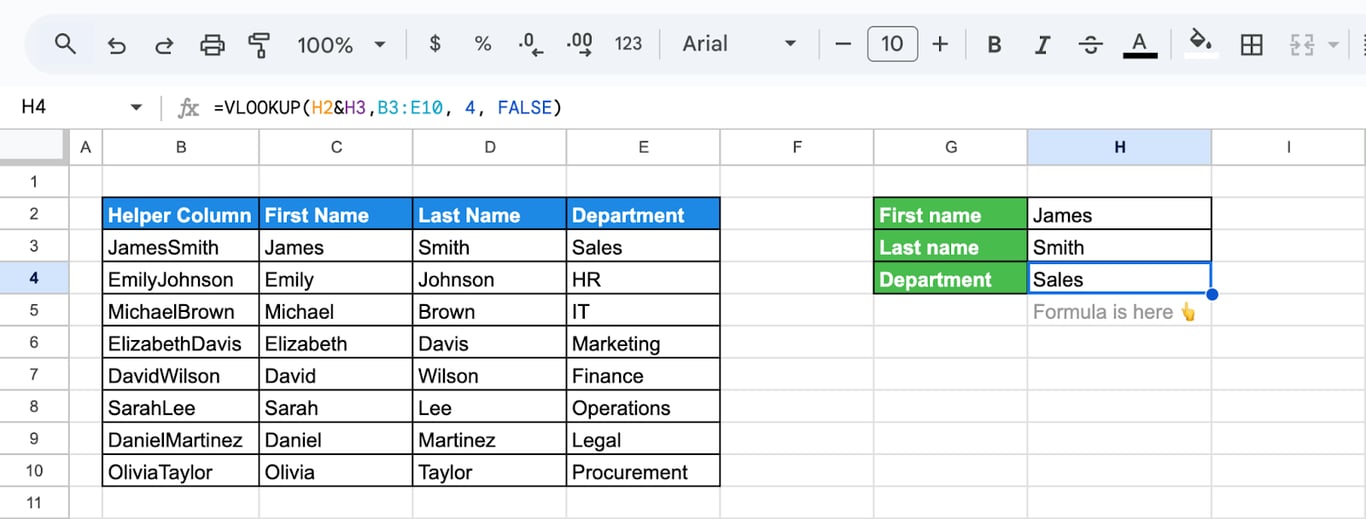
More approaches, including ones without a helper column, are in the guide to VLOOKUP with multiple criteria.
VLOOKUP from another sheet
To search a table on another tab of the same file, put the tab name and an exclamation mark before the range. The Employees tab holds IDs, names and hourly pay:
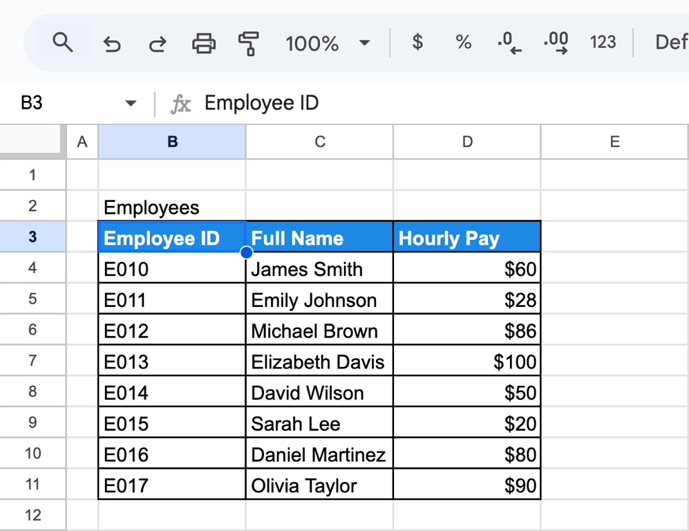
On another tab, this formula returns the hourly pay for the ID in B4:
=VLOOKUP(B4, Employees!$B$4:$D$11, 3, FALSE)
- B4: the employee ID on the current tab.
- Employees!$B$4:$D$11: the range on the Employees tab.
- 3: the third column of that range, the hourly pay.
- FALSE: exact match.
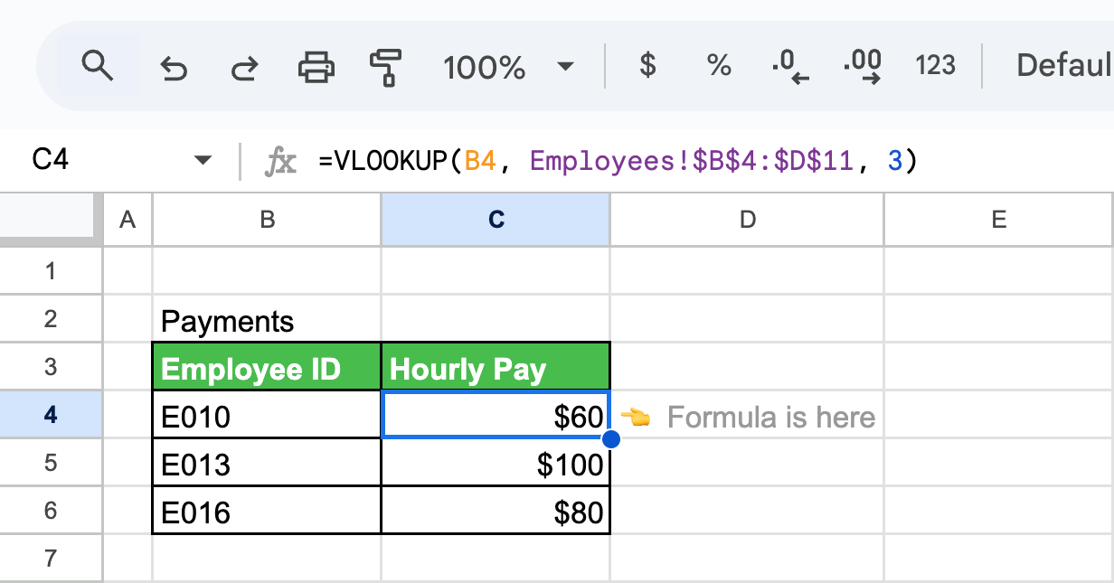
The formula in the screenshot leaves out FALSE. It returns the right values there only because the IDs in the Employees tab are sorted; with unsorted data it would not.
If the tab name contains spaces, put it in single quotes: 'Employee list'!$B$4:$D$11. The easiest way to get the reference right is to type the formula up to the range, then click the other tab and select the range with the mouse.
VLOOKUP from another spreadsheet
VLOOKUP from another spreadsheet
For a table in a different file, wrap the range in IMPORTRANGE, which takes the URL of the other spreadsheet and the range as text:
=VLOOKUP(B2, IMPORTRANGE("https://docs.google.com/spreadsheets/d/spreadsheet_id/edit", "Employees!B4:D11"), 3, FALSE)
- B2: the key to look for.
- IMPORTRANGE(…): the range B4:D11 of the Employees tab in the other file. Replace the URL with the address of your source spreadsheet.
- 3: the third column of the imported range.
The first time the formula connects two files, it returns #REF! and asks you to allow access. Click the cell and choose Allow access. Inside IMPORTRANGE the range is plain text, so dollar signs are not needed.
VLOOKUP with other functions
Several columns at once with ARRAYFORMULA
Inside ARRAYFORMULA, VLOOKUP takes a list of keys and a list of column numbers in curly braces:
=ARRAYFORMULA(VLOOKUP(G4:G6, B3:E10, {2, 3, 4}, FALSE))
- G4:G6: the employee IDs to look up.
- B3:E10: the range with ID, full name, email and department.
- {2, 3, 4}: return the second, third and fourth columns.
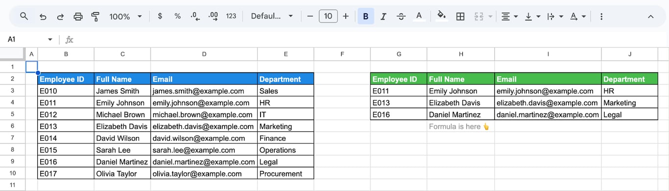
One formula fills a block of three rows and three columns.
A column chosen by its header with MATCH
A fixed index breaks when someone inserts a column into the table. MATCH finds the position of a header and passes it to VLOOKUP as the index:
=VLOOKUP(F3, B3:D10, MATCH(G2, B2:D2, 0), FALSE)
- F3: the employee ID.
- B3:D10: the range with ID, full name and department.
- MATCH(G2, B2:D2, 0): the position of the header named in G2 within the header row B2:D2. For “Department” it returns 3.
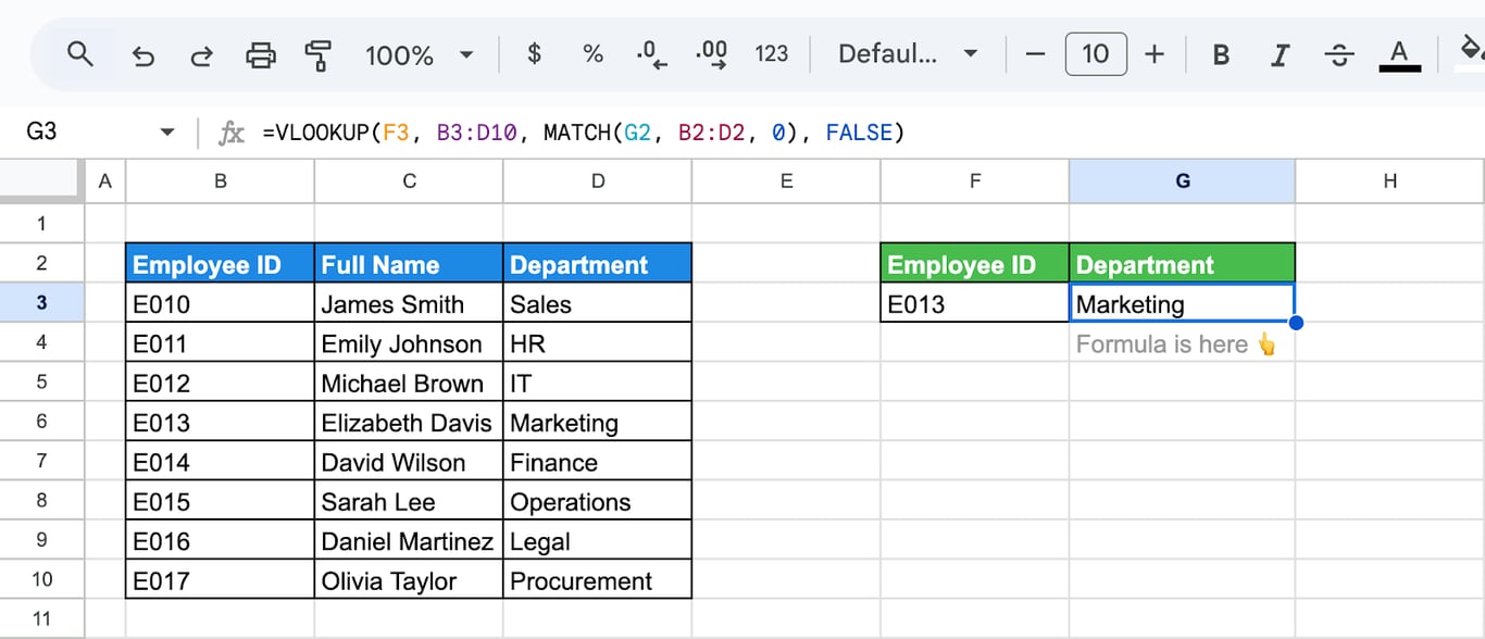
A message instead of #N/A
When the key is not in the table, VLOOKUP returns #N/A. IF with ISNA replaces it with your own text:
=IF(ISNA(VLOOKUP(F3, B3:D10, 3, FALSE)), "Employee Not Found", VLOOKUP(F3, B3:D10, 3, FALSE))
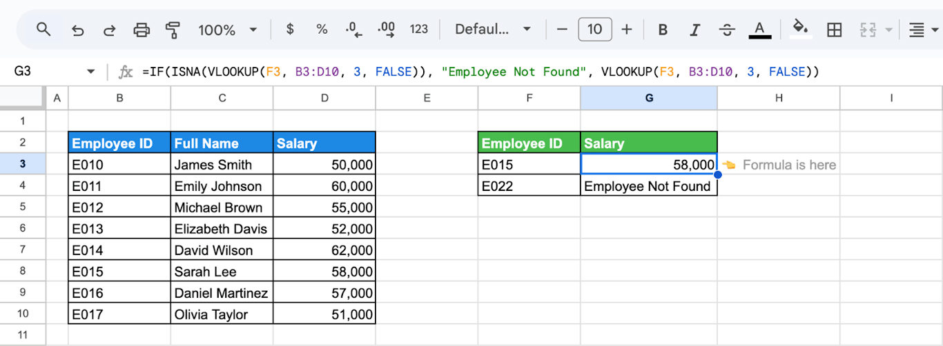
IFNA does the same with one lookup instead of two: =IFNA(VLOOKUP(F3, B3:D10, 3, FALSE), "Employee Not Found"). More combinations are in the guide to VLOOKUP with IF.
What VLOOKUP cannot do
- Look to the left. The key has to be in the first column of the range, and the returned column has to be to its right. To return a column on the left, use INDEX and MATCH,
=INDEX(B3:B12, MATCH("Mike", C3:C12, 0)), or XLOOKUP,=XLOOKUP("Mike", C3:C12, B3:B12). - Return more than one row. When the key appears several times, VLOOKUP returns the first match. For all matching rows use FILTER.
- Tell upper from lower case. “JOHN” and “John” are the same key.
- Search a row. For a table laid out sideways there is HLOOKUP.
VLOOKUP errors
⚠️ Error: #N/A although the value is in the table.
✅ Solution: Check three things. The key must be in the first column of the range. The two values must be of the same type: the number 1001 does not match the text “1001”. And there must be no extra spaces around either value; clean them with TRIM.
⚠️ Error: A wrong value, with no error.
✅ Solution: The last argument is missing or TRUE, and the first column is not sorted. Add FALSE.
⚠️ Error: #REF! with “evaluates to an out of bounds range”.
✅ Solution: The index is larger than the number of columns in the range. A range of two columns has no column 3.
⚠️ Error: #VALUE!
✅ Solution: The index is 0 or negative. Columns are counted from 1.
⚠️ Error: #NAME?
✅ Solution: The function name is misspelled, a text key is not in quotes, or a named range does not exist.
⚠️ Error: The formula breaks when it is copied down.
✅ Solution: The range moved with the formula. Lock it with dollar signs, $B$3:$D$10.
Related Google Sheets functions
Related Google Sheets functions
Functions that are often used with or instead of VLOOKUP, each with its own guide:
- XLOOKUP vs VLOOKUP: The newer lookup that searches in any direction.
- INDEX and MATCH: A lookup built from two functions.
- HLOOKUP: Searches for a value in the first row of a range and returns a value from the same column in a specified row.
- LOOKUP: Finds a value in a sorted row or column and returns the corresponding value from another range.
- QUERY vs VLOOKUP: When a query does the job better than a lookup.
- IMPORTRANGE: Brings a range from another spreadsheet into the current one.
- UNIQUE: Returns the distinct values of a range.
- Pivot tables: Summarize a table by category without formulas.
A VLOOKUP is a join that someone has to keep working
A VLOOKUP is a join that someone has to keep working
Each VLOOKUP attaches a column from one table to the rows of another: a price to an order, a manager to a region, a cost to a campaign. In a report built from exports, that join lives in formulas and depends on keys that two different systems have to spell the same way. One renamed campaign is enough to turn a row into #N/A, or into a silently wrong number when FALSE is missing.
The OWOX Data Marts extension for Google Sheets covers that half. A data analyst publishes a data mart (a table or an SQL query in your data warehouse) and makes it available for reports. In Sheets you open the extension, pick the data mart, tick the columns you want and run it. The rows land in a tab, ready for your formulas.
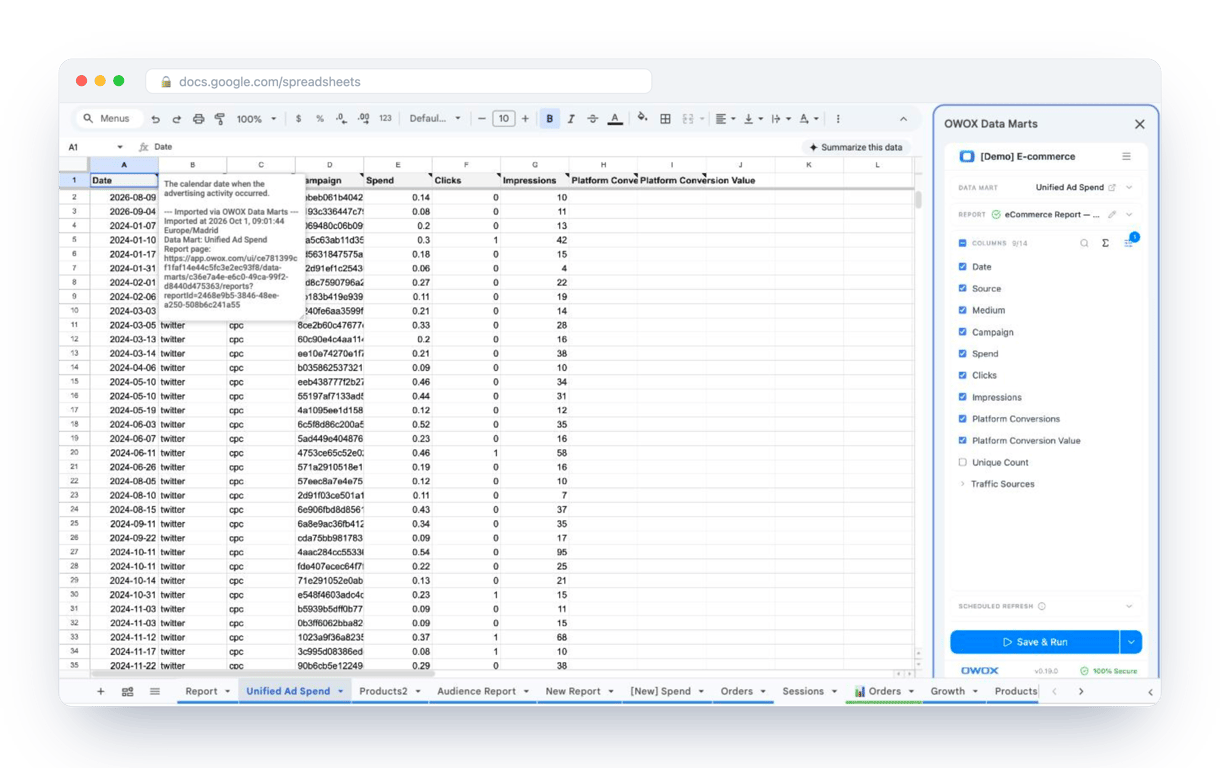
What changes for the person who maintains the sheet:
- Refresh replaces re-export. Refresh current report in the extension menu re-runs the same pull, and a scheduled refresh keeps the tab current without anyone touching it.
- The source is written on the sheet. The header cell of an imported tab carries a note with the data mart it came from, the time of the import and a link to the report.
- No SQL and no warehouse access needed. The analyst decides which data marts and columns are available. You choose from that list.
The extension does not write or change the analyst’s SQL. When the two tables are joined there once, with a real key, the sheet receives the matched columns on every refresh, and VLOOKUP is left for the small lookups that live only in the spreadsheet. Joined Data Marts in Google Sheets shows how that join is declared and where a joined report can still double-count. The extension comes with the OWOX Cloud plans of OWOX Data Marts; spreadsheet reporting describes both ways data reaches a sheet.
Turn your data into decisions.
Governed data marts give you the clean foundation ML needs to actually work.
- No AI hallucinations
- Analyst-governed definitions
- Every number traces to SQL
Frequently Asked Questions
How to use VLOOKUP to compare two lists in Google Sheets?
Look up each value of the first list in the second one and return the found value: =VLOOKUP(A2, D$2:D$100, 1, FALSE). Values that exist in both lists are returned, missing ones show #N/A. Wrap it in IF and ISNA to get a label: =IF(ISNA(VLOOKUP(A2, D$2:D$100, 1, FALSE)), "Missing", "Found").
How do you handle case-sensitive lookups using VLOOKUP in Google Sheets?
VLOOKUP in Google Sheets is not case-sensitive. To perform a case-sensitive lookup, you can use a combination of functions like EXACT or helper columns to convert text to a consistent case.
Can VLOOKUP search for values vertically and horizontally in Google Sheets?
No. VLOOKUP searches vertically: it looks down the first column of a range and returns a value from the same row. For a table laid out in rows, use HLOOKUP, which searches along the first row. XLOOKUP and INDEX with MATCH work in both directions.
How do you specify the range for a VLOOKUP search in Google Sheets?
You set the range for a VLOOKUP search by indicating the sheet name, if applicable, followed by an exclamation mark (!), and then providing the cell range within which you want to search.
How do you reference data from another tab in Google Sheets using VLOOKUP?
Put the tab name and an exclamation mark before the range: =VLOOKUP(A2, Employees!$A$2:$C$50, 3, FALSE). If the tab name contains spaces, wrap it in single quotes: 'Employee list'!$A$2:$C$50.
How do you modify VLOOKUP to search from right to left in Google Sheets?
VLOOKUP in Google Sheets searches from left to right. If you need to search from right to left, you can use the INDEX and MATCH functions combined.
What is VLOOKUP in Google Sheets used for?
VLOOKUP in Google Sheets is used to search for a specified value in a column, and when found, retrieve information from the same row in a different column. It's commonly used for data analysis, lookup operations, and organizing information.
Is it possible to use VLOOKUP to search data from another sheet in Google Sheets?
Yes, VLOOKUP can search data from another sheet in Google Sheets. You need to select the range using the sheet name, followed by an exclamation mark (!), and then the cell range.
What does the "column index number" mean in a VLOOKUP formula?
The "column index number" in a VLOOKUP formula refers to the column from which you want to retrieve data. It shows the relative position of the column within the specified range.