DAY, DAYS and DAYS360 in Google Sheets: formulas and examples
DAY returns the day of the month of a date, DAYS the number of days between two dates, and DAYS360 the number of days on a 360-day year used in finance. This guide shows the syntax of each, the difference between the US and European methods of DAYS360, and examples with IF, VLOOKUP and conditional formatting.
Three functions with similar names do three different jobs:
| Function | Returns | Example | Result |
|---|---|---|---|
DAY(date) |
The day of the month, 1 to 31 | =DAY(DATE(2024,6,30)) |
30 |
DAYS(end_date, start_date) |
The number of days between two dates | =DAYS(DATE(2024,6,30), DATE(2024,4,1)) |
90 |
DAYS360(start_date, end_date, [method]) |
The number of days between two dates on a year of twelve 30-day months | =DAYS360(DATE(2024,4,1), DATE(2024,6,30)) |
89 |
Note the order of the arguments: DAYS takes the end date first, DAYS360 the start date first.
DAY: the day of the month
=DAY(date)
- date: a date, a cell with a date, or a function that returns one.
=DAY(B3)
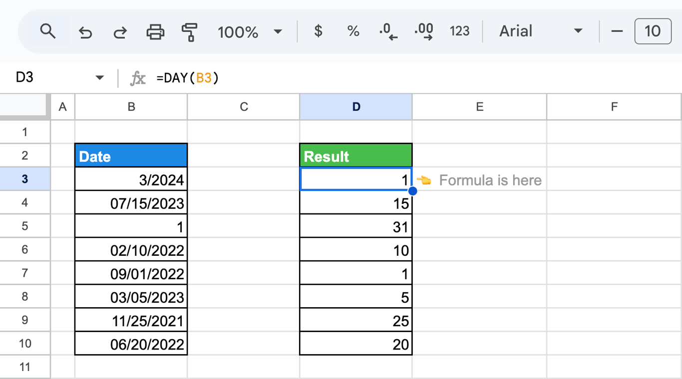
DAY reads the day number and drops the month and the year. Row 5 of the screenshot shows what happens with a plain number: a date in Sheets is a count of days from 30 December 1899, so the number 1 is 31 December 1899, and DAY returns 31. A text that is not a date returns #VALUE!. The companion functions are MONTH and YEAR.
The number of days in a month
=DAY(EOMONTH(A2, 0))
EOMONTH returns the last day of the month of the date in A2, and DAY its number: 29 for February 2024, 31 for March.
Flag a day of the month with IF
=IF(DAY(B3) = 1, "First Day", "Not First")
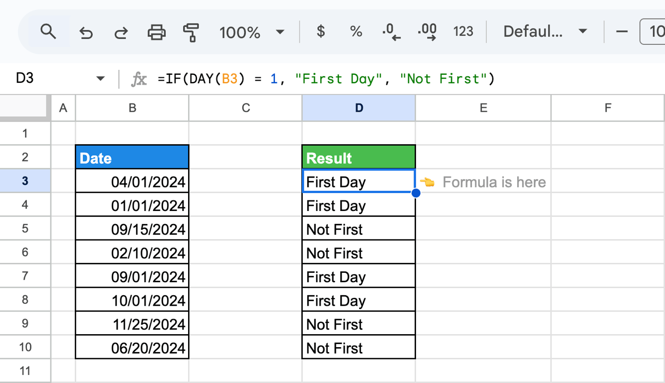
The same test works for the middle or the end of the month: DAY(B3) = 15, or B3 = EOMONTH(B3, 0) for the last day. More on conditions in the guide to IF.
Highlight dates with conditional formatting
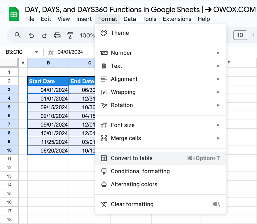
- Select the dates, here B3:C10.
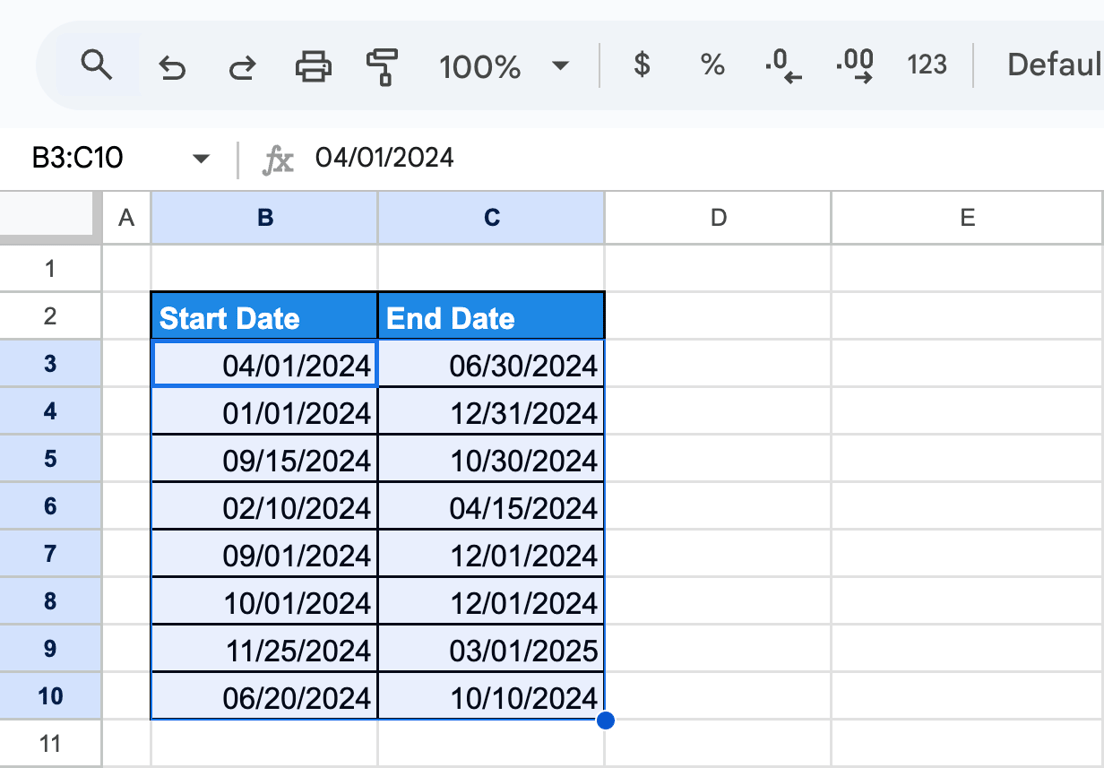
- Click Format > Conditional formatting.
- Under Format cells if, choose Custom formula is, enter the formula and pick a fill color:
=DAY(B3) > 15
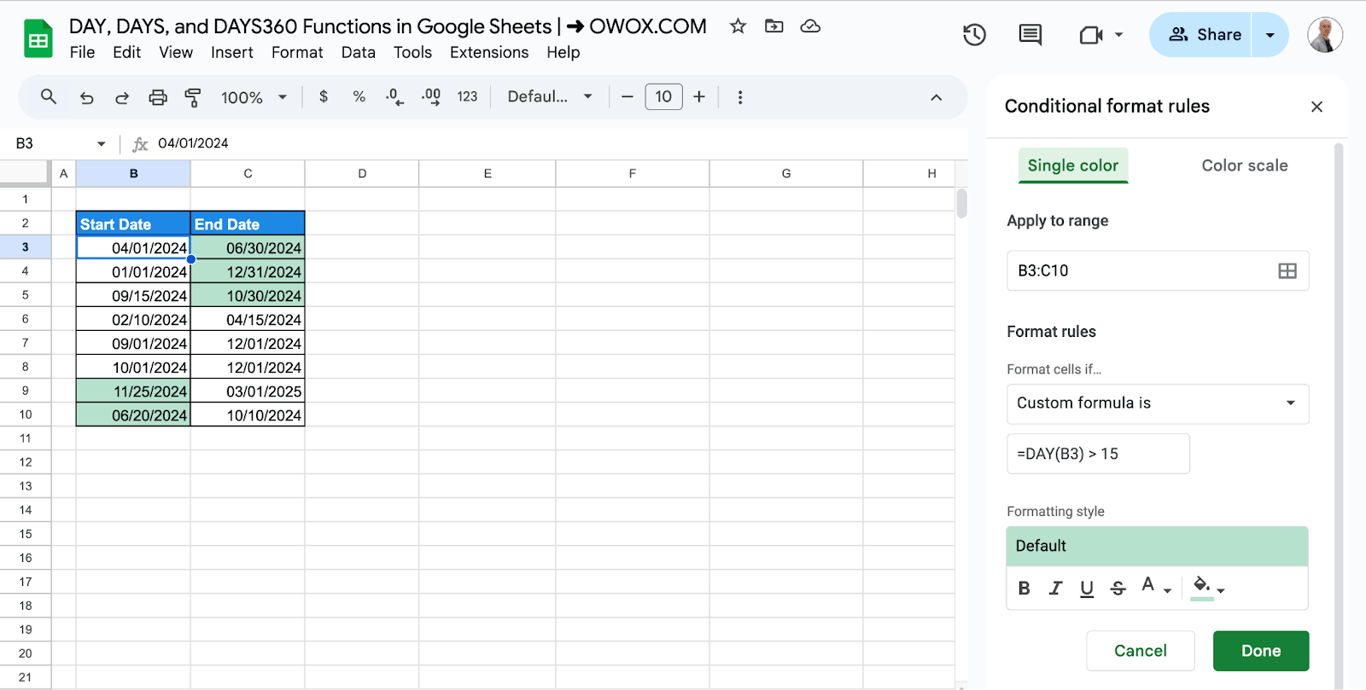
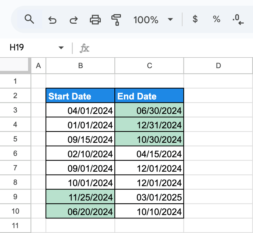
The formula is written for the first cell of the range and Sheets applies it to every other cell in turn. All dates in the second half of a month are shaded:
Count the dates that fall on a given day
=SUMPRODUCT(DAY(B3:B10) = 1)
DAY is calculated for every date in the range, and SUMPRODUCT counts the rows where the result is 1. With a helper column that already holds the day numbers, a plain COUNTIF does the same:
=COUNTIF(B3:C10, DAY(B3))
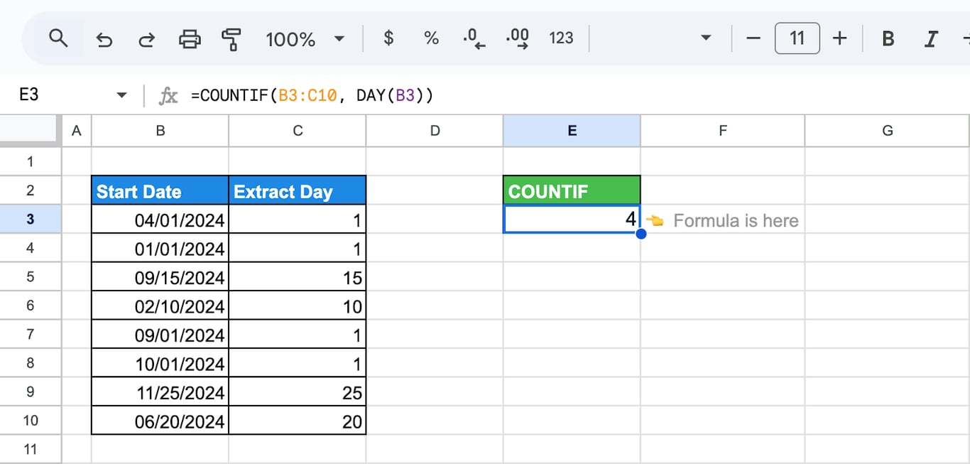
DAY(B3) is 1, and four cells of the helper column hold a 1. See COUNTIF and COUNTIFS.
Age from a birth date
=YEAR(TODAY()) - YEAR(C3) - (TODAY() < DATE(YEAR(TODAY()), MONTH(C3), DAY(C3)))
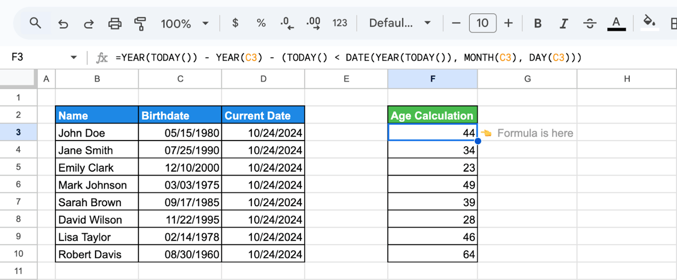
The formula subtracts the years and takes one more off if this year’s birthday has not come yet. DATEDIF does the same in one step: =DATEDIF(C3, TODAY(), "Y"). See the guide to DATE functions.
DAYS: the number of days between two dates
DAYS: the number of days between two dates
=DAYS(end_date, start_date)
=DAYS(C3, B3)
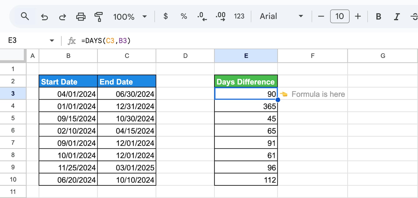
The result is the same as subtracting the dates, =C3-B3: both count the real calendar days, leap days included. If the end date is earlier than the start date, the result is negative. Times are ignored, only whole days count.
Dates can be typed into the formula as text in the format of the spreadsheet’s locale, or built with DATE, which works in any locale:
=DAYS("4/1/2024", DATE(2023, 12, 31))
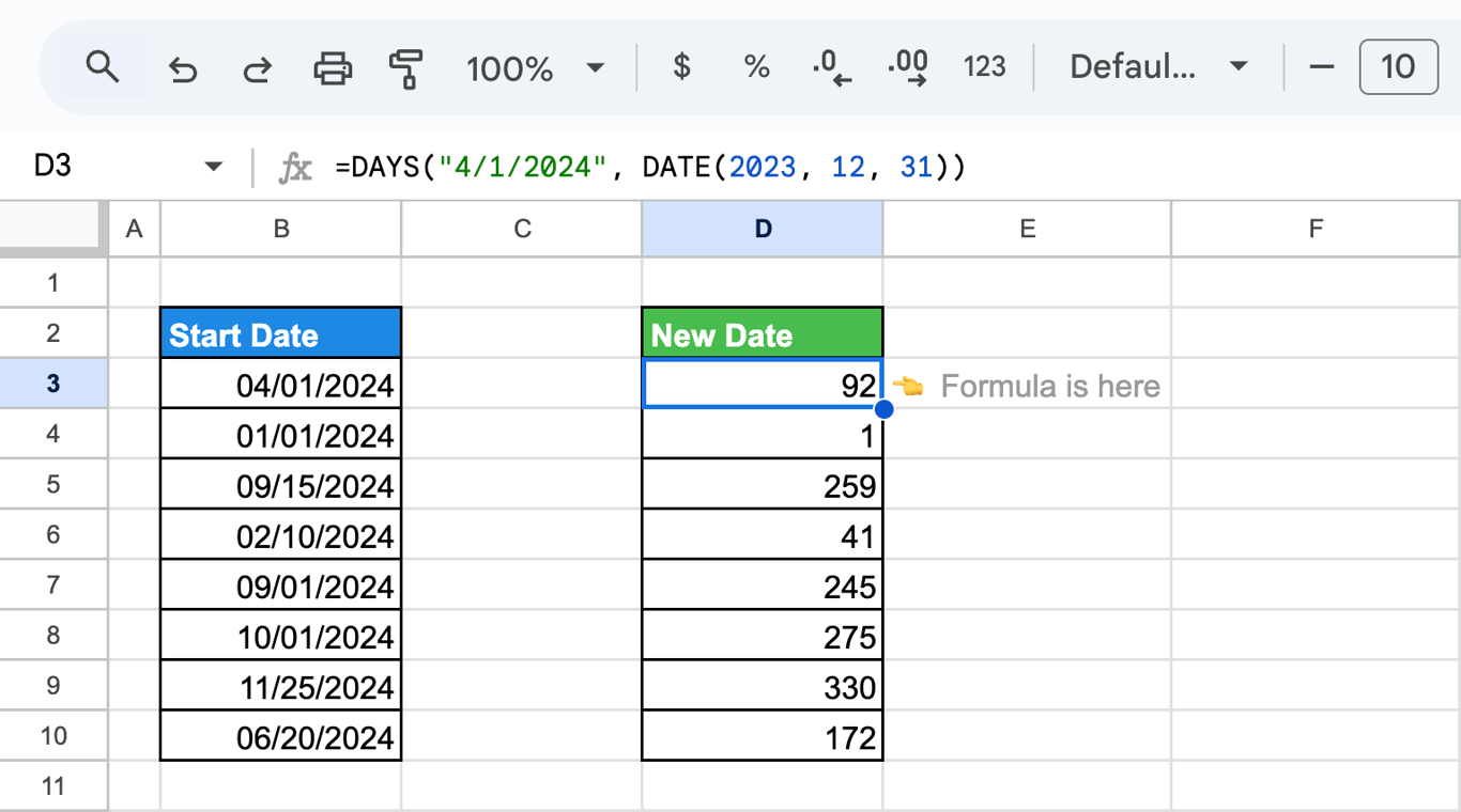
A common mistake: subtracting DAY from DAY
=DAY(C3)-DAY(B3)
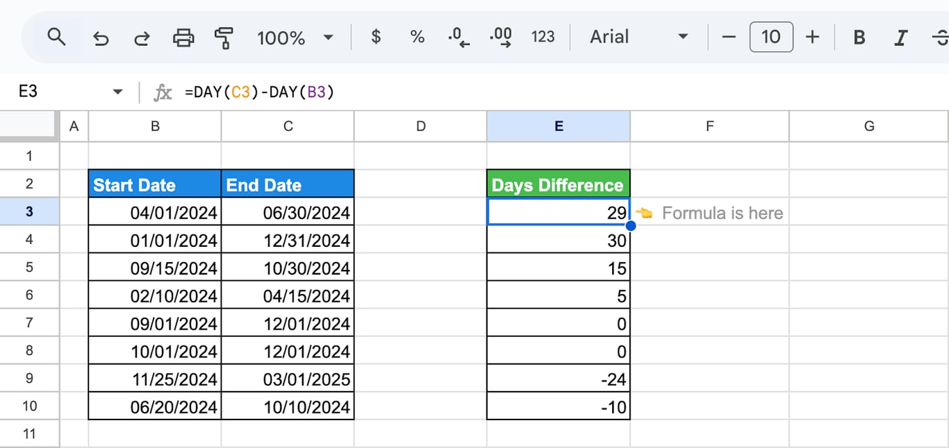
This subtracts one day number from another and ignores months and years: from 1 April to 30 June it returns 29, although 90 days passed, and it goes negative when the end date has a smaller day number. To count days between dates, use DAYS or subtract the dates themselves.
Days left until a deadline
=DAYS(C3, TODAY())
The result is positive before the deadline, 0 on the day and negative after it. To turn the number into a status, look it up in a table of thresholds with an approximate match:
=VLOOKUP(DAYS(C3, TODAY()), $B$13:$C$18, 2, TRUE)
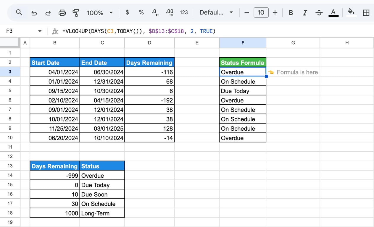
The threshold table must be sorted in ascending order. Each status applies from its number up to the next one, so in this table “Due Today” covers 0 to 9 days and “Due Soon” 10 to 29; rename or move the thresholds to fit your process. TODAY is recalculated every day, so the statuses update themselves. See VLOOKUP for the approximate match.
For working days only, use NETWORKDAYS.
OWOX Data Marts
See your first report built in real time. 15 minutes.
- Connect your data warehouse
- Pick your metrics
- Get a live Google Sheets report
In the time it takes to write a ticket. Then imagine never writing that ticket again.
Book a DemoWe'll use your actual use case
DAYS360: days on a 360-day year
DAYS360: days on a 360-day year
=DAYS360(start_date, end_date, [method])
- start_date, end_date: the two dates, start first.
- method: optional. FALSE or omitted is the US method, TRUE the European method.
DAYS360 treats every month as 30 days and the year as 360. Some loans, bonds and accounting systems calculate interest this way, because every month then carries the same weight. Use it when a contract or a rule names the 30/360 convention, and DAYS for everything else.
=DAYS360(B3, C3, FALSE)
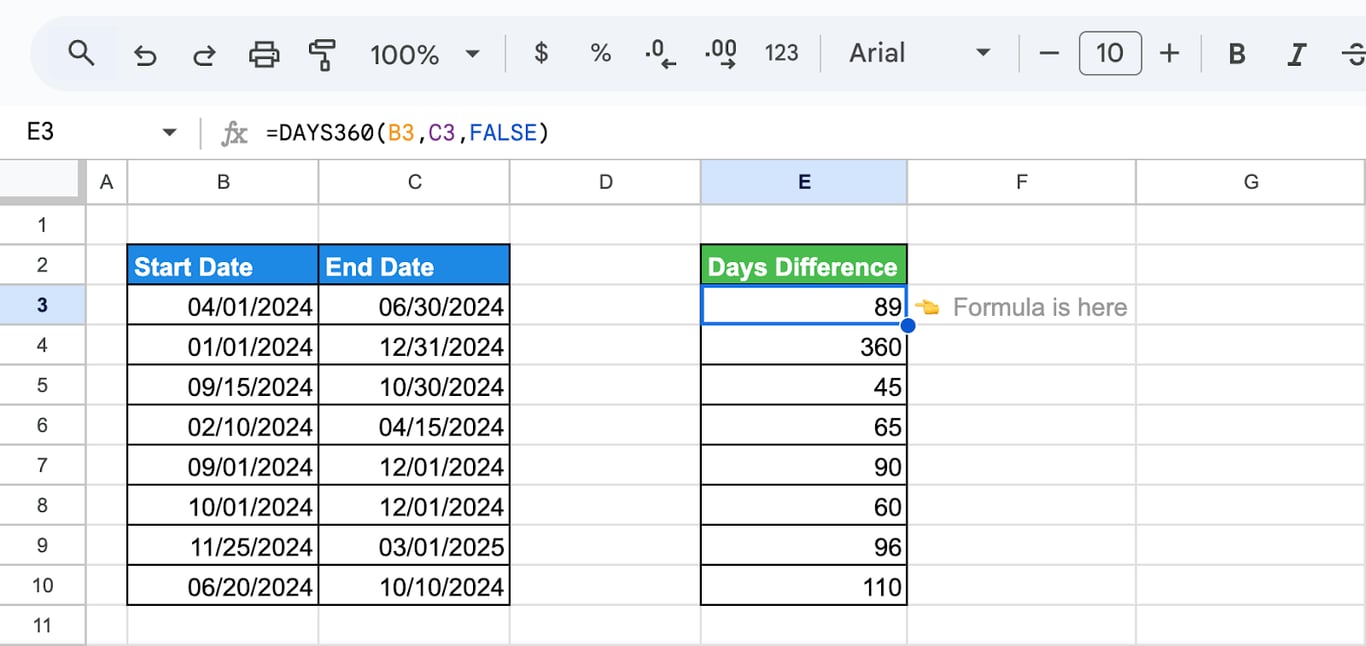
Compare with DAYS in the screenshot above: 1 April to 30 June is 90 real days and 89 on the 360-day year; 1 January to 31 December is 365 and 360.
US and European methods
The two methods differ in how they treat the 31st and the end of February:
- US (FALSE): an end date on the 31st becomes the 1st of the next month, unless the start date is the 30th or 31st, in which case it becomes the 30th. A start date on the 31st or on the last day of February counts as the 30th.
- European (TRUE): every 31st becomes the 30th. February is left as it is.
=DAYS360(B3, C3, TRUE)
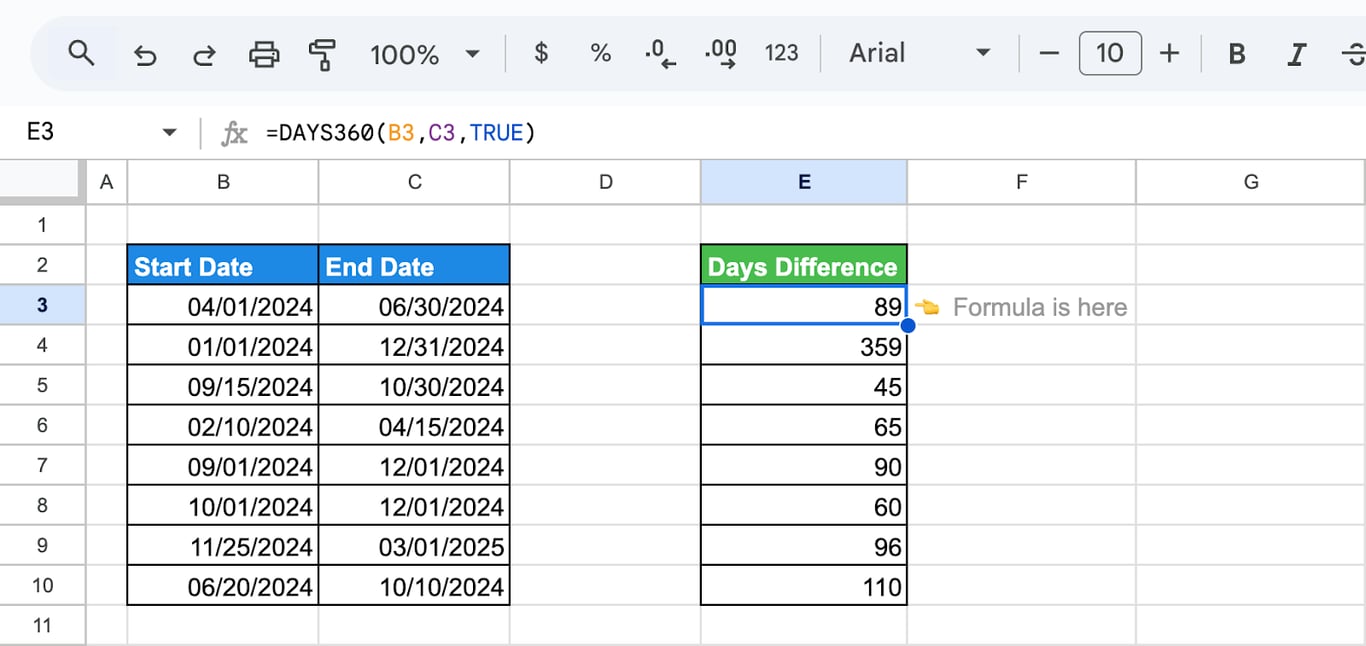
| Start | End | US method | European method |
|---|---|---|---|
| 1 January 2024 | 31 December 2024 | 360 | 359 |
| 29 February 2024 | 31 March 2024 | 30 | 31 |
For most pairs of dates the two methods agree. Which one applies is set by the contract, not by preference.
Interest on a 360-day and a 365-day year
Simple interest is the principal times the annual rate times the days, divided by the days in the year. The divisor changes the result:
=(B3*C3*D3)/360
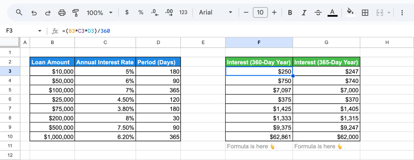
=(B3*C3*D3)/365
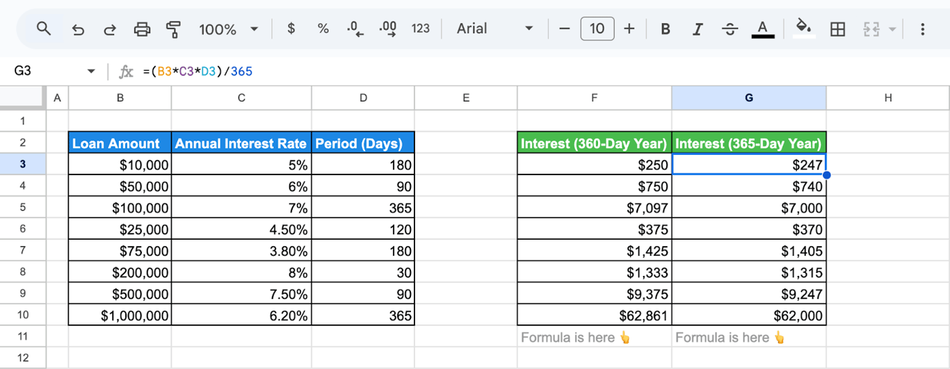
Dividing by 360 gives a slightly higher interest for the same number of days: 250 against 247 on the first loan, and 62,861 against 62,000 on the last.
Errors with DAY, DAYS and DAYS360
Errors with DAY, DAYS and DAYS360
⚠️ Error: #VALUE!
✅ Solution: An argument is a text that Sheets cannot read as a date, such as “abc” or a date typed in the format of another locale, or the method of DAYS360 is not TRUE or FALSE. Build dates with DATE(year, month, day).
⚠️ Error: DAYS returns a negative number.
✅ Solution: The arguments are swapped. DAYS takes the end date first; DAYS360 takes the start date first.
⚠️ Error: DAY returns 30 or 31 for an empty cell or a small number.
✅ Solution: An empty cell is 0 and a number is a count of days from 30 December 1899, so DAY returns the day of a date in 1899 or 1900. Test the cell first: =IF(B3="", "", DAY(B3)).
⚠️ Error: The result shows as a date, such as 30/01/1900, where a number was expected.
✅ Solution: The cell has a date format. Apply Format > Number > Number.
⚠️ Error: DAYS360 and DAYS give different results.
✅ Solution: They are supposed to. DAYS360 counts 30 days in every month. For real calendar days use DAYS.
⚠️ Error: The day and the month are swapped.
✅ Solution: A text date such as “4/1/2024” is read according to the spreadsheet’s locale: 1 April in the United States, 4 January in most of Europe. See the guide to dates and times.
Related Google Sheets functions
Related Google Sheets functions
- DATE functions: DATE, EDATE, DATEVALUE and DATEDIF.
- MONTH and EOMONTH: The month of a date and the last day of a month.
- YEAR and YEARFRAC: The year of a date and the fraction of a year between two dates.
- WORKDAY and NETWORKDAYS: Working days between dates.
- NOW and TODAY: The current date and time.
- Dates and times: How Sheets stores dates.
- Date filtering with QUERY: Rows from a date range.
Day counts are only as right as the dates under them
Day counts are only as right as the dates under them
A formula with TODAY recalculates every morning, but the dates it compares with do not refresh themselves. If the deadlines or order dates in the sheet come from an export, “days remaining” is measured against whatever was true on the day of the export. The arithmetic is correct and the answer is still out of date.
The OWOX Data Marts extension for Google Sheets covers that half. A data analyst publishes a data mart (a table or an SQL query in your data warehouse) and makes it available for reports. In Sheets you open the extension, pick the data mart, tick the columns you want and run it. The rows land in a tab, ready for your formulas.
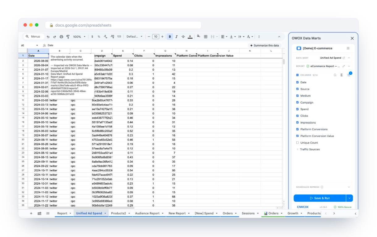
What changes for the person who maintains the sheet:
- Refresh replaces re-export. Refresh current report in the extension menu re-runs the same pull, and a scheduled refresh keeps the tab current without anyone touching it.
- The source is written on the sheet. The header cell of an imported tab carries a note with the data mart it came from, the time of the import and a link to the report.
- No SQL and no warehouse access needed. The analyst decides which data marts and columns are available. You choose from that list.
The extension does not write or change the analyst’s SQL. DAY, DAYS and DAYS360 then count from the dates as they are now, not as they were at the last paste. The extension comes with the OWOX Cloud plans of OWOX Data Marts; spreadsheet reporting describes both ways data reaches a sheet.
Turn your data into decisions.
Governed data marts give you the clean foundation ML needs to actually work.
- No AI hallucinations
- Analyst-governed definitions
- Every number traces to SQL
Frequently Asked Questions
What errors should I watch out for when using the DAYS360 function?
When using DAYS360, watch for errors due to non-date inputs or improper formatting. Also, remember it approximates each month as 30 days, which may cause inaccuracies for actual month lengths, particularly in financial calculations involving leap years or different month lengths.
What is the correct way to use the DAY function with other formulas?
The DAY function can be combined with other formulas for more complex calculations. For example, =IF(DAY(A1)=15, "Mid-month", "Other") checks if a date is the 15th and returns "Mid-month." You can also use it for conditional calculations or date manipulations.
How can I highlight specific days using conditional formatting?
To highlight specific days in Google Sheets using conditional formatting, select the range, go to Format > Conditional formatting, then set a custom formula like =DAY(A1)=15 to highlight cells where the day is 15. Adjust the formatting style as needed.
What is the difference between DAYS360 and DAYS functions?
The DAYS function calculates the actual number of days between two dates. The DAYS360 function, however, uses a 360-day year (twelve 30-day months) for calculations, which is useful for financial purposes where standardized month lengths are needed for consistency.
What does the DAY function in Google Sheets do?
The DAY function in Google Sheets extracts the day of the month (1-31) from a given date. For example, =DAY("2024-10-03") returns 3. It helps when you need to analyze or manipulate date data based on the day component.
How do I calculate the number of days between two dates in Google Sheets?
You can use the DATEDIF function to calculate the number of days between two dates. The syntax is:=DATEDIF(start_date, end_date, "D")Here, "D" stands for days. For example: =DATEDIF(A1, B1, "D")It will return the number of days between the dates in cells A1 and B1.