QUERY with CONCATENATE in Google Sheets: how to concatenate two columns
The QUERY language cannot join columns: select A & B returns an error. This guide shows the three ways that work: concatenate the columns before the query, join the columns of the query result, or collect the result into one cell, plus the simpler formulas for cases where no QUERY is needed.

The QUERY language in Google Sheets has no concatenation operator: "select B & C" returns #VALUE!. To concatenate two columns in a QUERY, join them before the query, inside curly braces, and wrap the formula in ARRAYFORMULA:
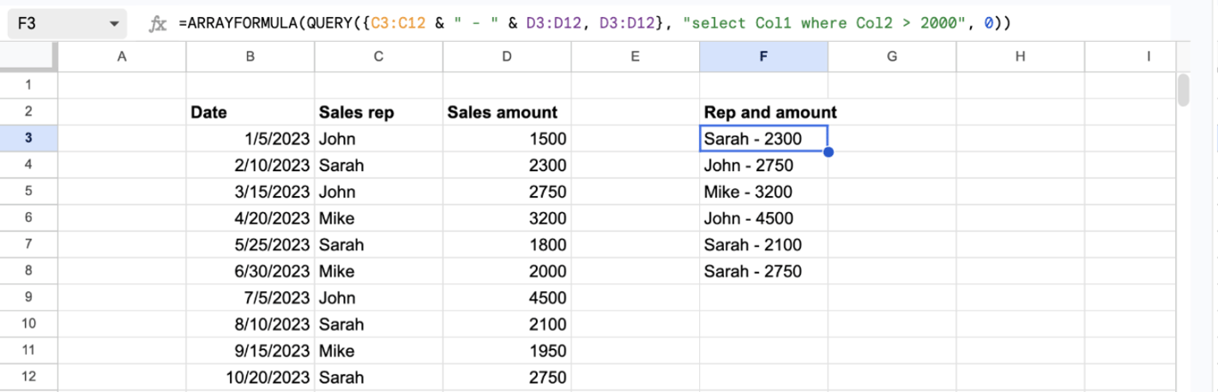
=ARRAYFORMULA(QUERY({C3:C12 & " - " & D3:D12, D3:D12}, "select Col1 where Col2 > 2000", 0))
The formula returns one column, sales rep and amount joined with a dash, for the rows where the amount is above 2,000.
There are three ways to combine the two functions, depending on where the join happens:
| You need | Approach |
|---|---|
| A joined column that the query can also filter or sort by | Concatenate before the query |
| The columns of the query result joined row by row | Join after the query |
| All rows of the query result in one cell | TEXTJOIN around the query |
What each function does
=QUERY(data, query, [headers])
QUERY filters, sorts and summarizes a range with a query string. Its language can select columns, compare them and aggregate them, but it cannot build a new text value from two columns.
=CONCATENATE(string1, [string2, ...])
CONCATENATE joins text. The ampersand (&) does the same and is shorter: =B3 & " " & C3.
Concatenate before the query
Build the joined column first and hand it to QUERY as part of the data:
=ARRAYFORMULA(QUERY({C3:C12 & " - " & D3:D12, D3:D12}, "select Col1 where Col2 > 2000", 0))
- {C3:C12 & “ - “ & D3:D12, D3:D12}: a table built in the formula. Its first column is the joined text, its second column is the amount.
- “select Col1 where Col2 > 2000”: when the data is built in curly braces and not taken from the sheet, columns are named Col1, Col2 and so on, in the order they appear in the braces. Letters such as C and D do not work here.
- 0: the data has no header row.
- ARRAYFORMULA: makes the ampersand work on the whole range. Without it the formula returns an error.
Because the joined column is part of the data, the query can use it like any other column: sort by it with order by Col1, or filter it with where Col1 contains 'Sarah'.
OWOX Data Marts
See your first report built in real time. 15 minutes.
- Connect your data warehouse
- Pick your metrics
- Get a live Google Sheets report
In the time it takes to write a ticket. Then imagine never writing that ticket again.
Book a DemoWe'll use your actual use case
Join the columns of the query result
Join the columns of the query result
The second way runs the query first and joins its columns afterwards.
All columns of each row
This formula joins the cells of every row with a space:
=TRANSPOSE(QUERY(TRANSPOSE(B3:C12),,6^6))
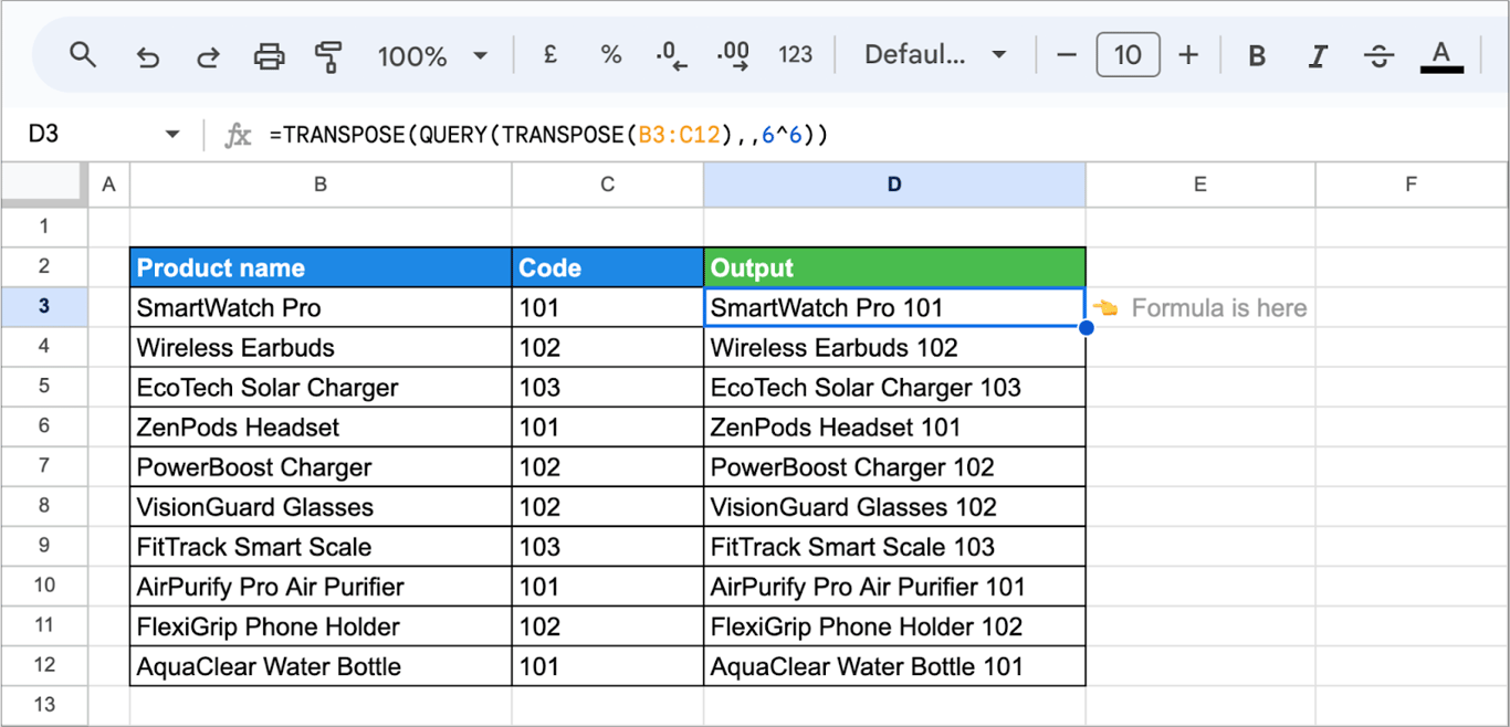
It relies on the third argument of QUERY, the number of header rows. When a range has several header rows, QUERY merges them into one, with a space between the values. The formula turns that into a join:
- TRANSPOSE(B3:C12): flips the range, so each row becomes a column.
- QUERY(…, , 6^6): no query string, and 6^6 (46,656) header rows, more than the data has. QUERY treats every row as a header and merges each column into a single cell.
- TRANSPOSE: flips the result back into a column.
Only the rows that match a condition
Put a query inside to filter the rows first. This formula keeps the products with the code 101, joins name and code, and replaces the spaces with underscores:
=ARRAYFORMULA(SUBSTITUTE(TRIM(TRANSPOSE(QUERY(TRANSPOSE(QUERY(B3:C12, "select * where C contains '101'")),,COLUMNS(QUERY(B3:C12, "select * where C contains '101'"))))), " ", "_"))
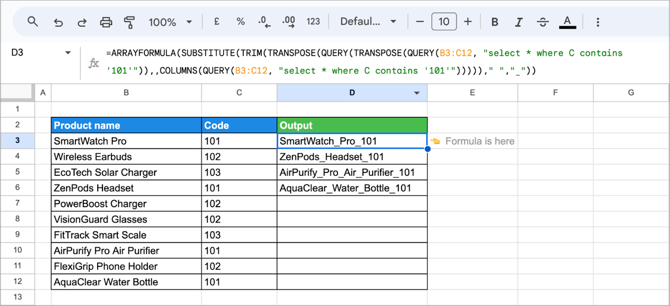
- QUERY(B3:C12, “select * where C contains ‘101’”): the rows with the code 101.
- TRANSPOSE and the outer QUERY: the header-row join from the previous example.
- TRIM: removes extra spaces.
- SUBSTITUTE(…, “ “, “_”): replaces every space with an underscore, including the spaces inside product names: SmartWatch Pro becomes SmartWatch_Pro.
A shorter formula for the same job uses BYROW, which applies a function to each row of the query result, and TEXTJOIN, which takes the separator as an argument:
=BYROW(QUERY(B3:C12, "select * where C contains '101'", 0), LAMBDA(row, TEXTJOIN("_", TRUE, row)))
Here the separator goes only between the columns, and the product names keep their spaces.
Collect the query result into one cell
Collect the query result into one cell
To list the values a query returns in a single cell, wrap the query in TEXTJOIN:
=TEXTJOIN(", ", TRUE, QUERY(C3:D12, "select C where D > 2000", 0))
- “, “: the separator.
- TRUE: skip empty cells.
- QUERY(…): the sales reps whose amount is above 2,000.
The result is one cell: Sarah, John, Mike, John, Sarah, Sarah. JOIN works the same way for a single column: =JOIN(", ", QUERY(C3:D12, "select C where D > 2000", 0)).
When you do not need QUERY
If there is nothing to filter, sort or aggregate, the join is simpler without QUERY.
ARRAYFORMULA with an ampersand
=ARRAYFORMULA(B3:B12 & "_" & C3:C12)
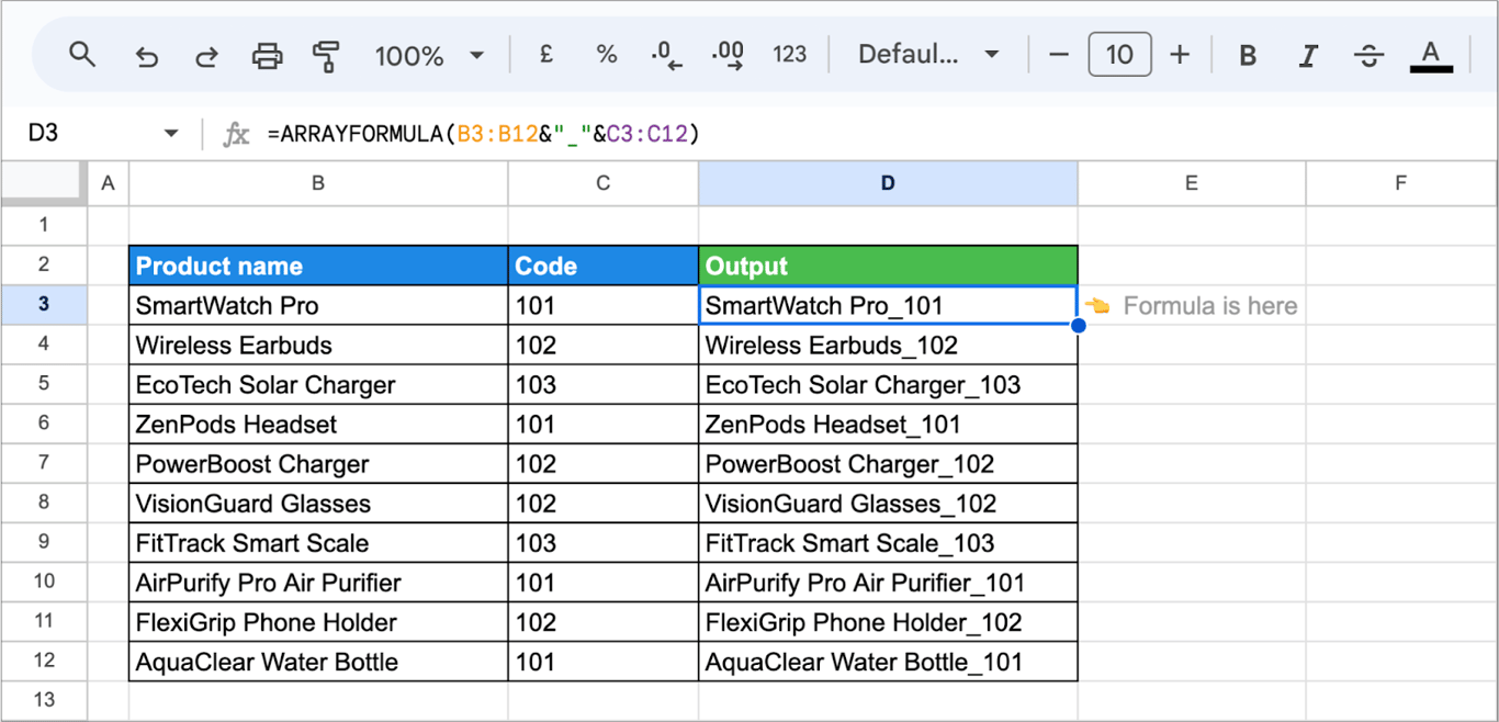
One formula in the first cell joins the two columns for every row. See the guide to ARRAYFORMULA for how this works.
CONCATENATE for one row
=CONCATENATE(B3, " ", C3)
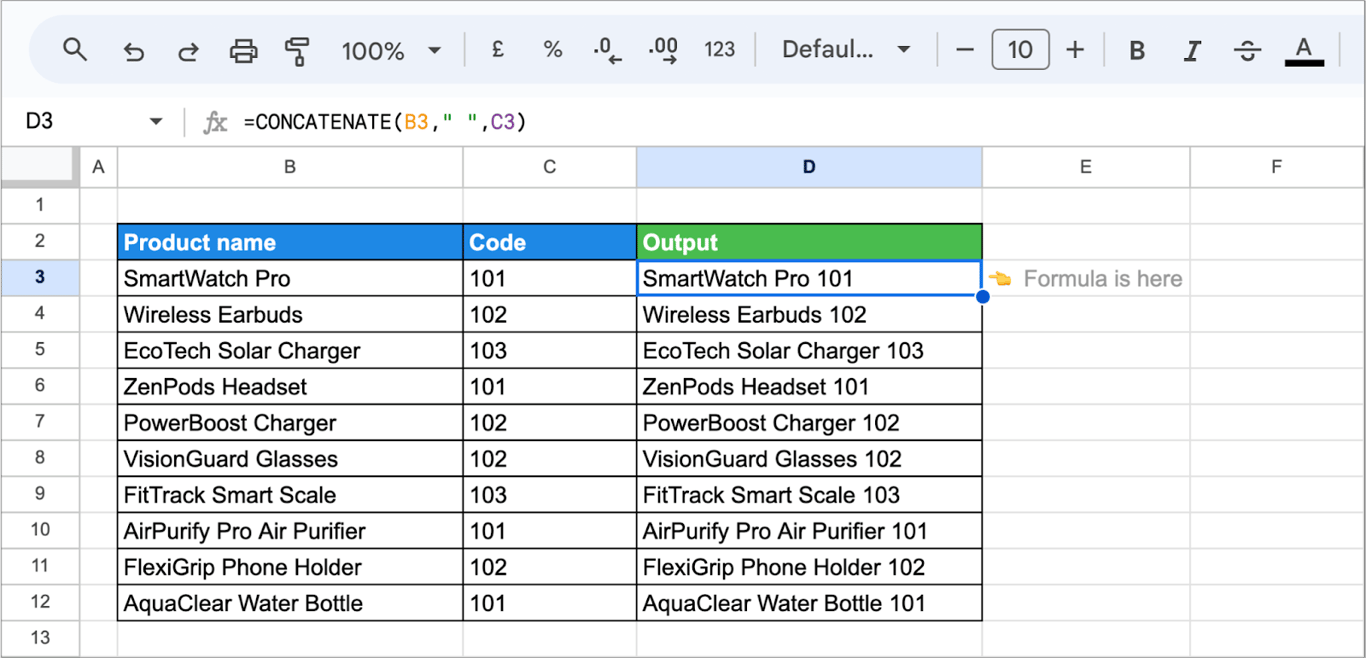
CONCATENATE joins the cells you list, with the separators you put between them. Copy the formula down for the other rows.
IF with CONCATENATE for a condition
=IF(C3=101, CONCATENATE(C3, "_", B3), "")
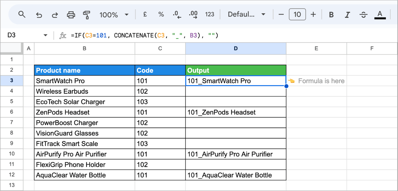
IF joins the code and the name only where the code equals 101 and leaves the other cells empty.
ARRAYFORMULA with CONCAT
=ARRAYFORMULA(CONCAT(B3:B12, C3:C12))
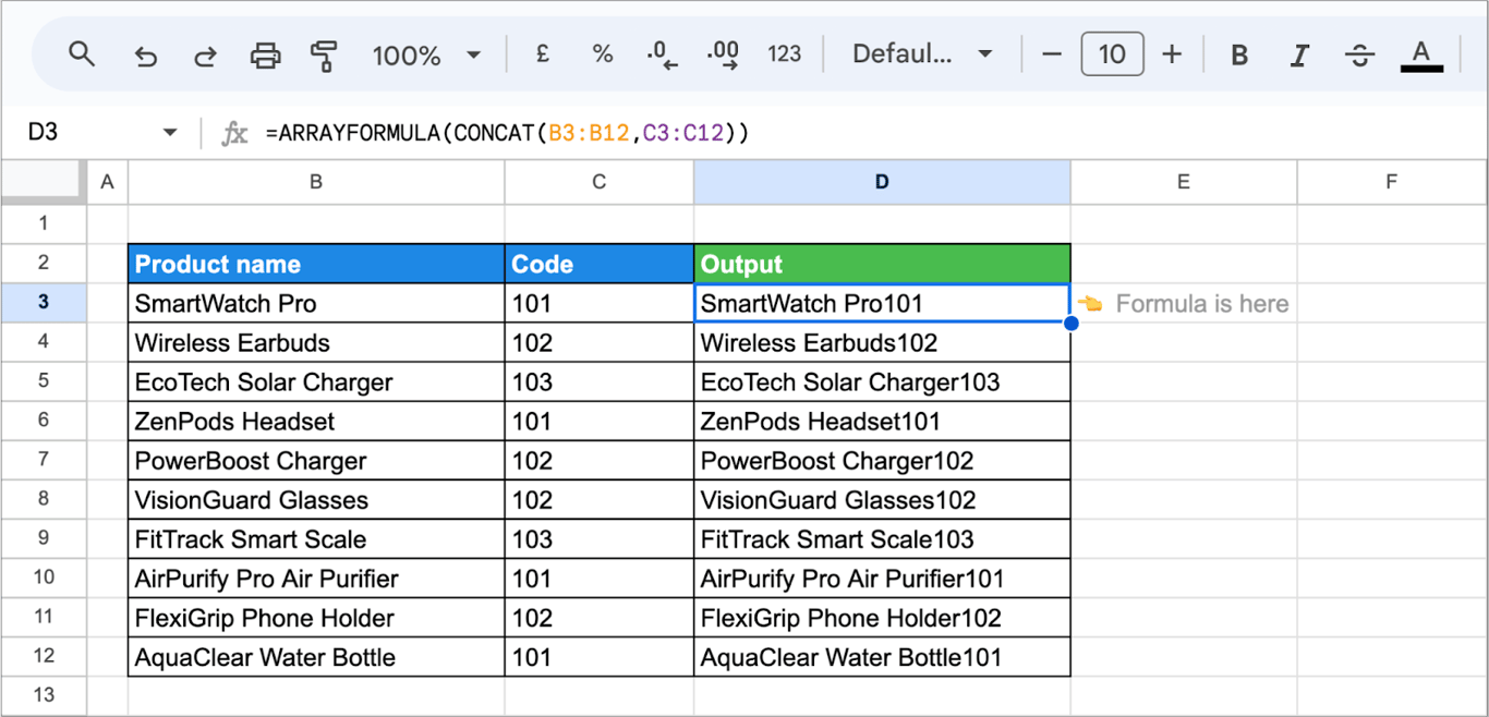
CONCAT joins exactly two values and has no room for a separator, so the result runs together: SmartWatch Pro101. Use the ampersand when you need a separator.
Errors and how to fix them
⚠️ Error: #VALUE! for a query such as "select B & C".
✅ Solution: The query language has no & operator and no CONCATENATE. Join the columns before the query, in curly braces, or after it.
⚠️ Error: The formula with curly braces returns an error.
✅ Solution: Check two things. The formula has to be wrapped in ARRAYFORMULA, and the query has to use Col1, Col2 instead of column letters.
⚠️ Error: Formula parse error after pasting a formula from a web page or a document.
✅ Solution: The quotes were replaced with typographic ones (“ ” or ‘ ’). Retype them as straight quotes in the formula bar.
⚠️ Error: The joined values have double or trailing spaces.
✅ Solution: Empty cells in the range can leave a space behind. Wrap the result in TRIM.
Related Google Sheets functions
Related Google Sheets functions
Functions that are often used next to QUERY and CONCATENATE, each with its own guide:
- QUERY with IMPORTRANGE: Queries a range that lives in another spreadsheet.
- QUERY date filtering: Filters rows by a date or a date range inside a QUERY formula.
- FILTER: Extracts the rows that meet a condition, without a query string.
- VLOOKUP: Finds a value in a table by a key.
- XLOOKUP: A lookup that can search in any direction.
- Pivot tables: Summarize a table by category without formulas.
- REPT: Repeats text a set number of times.
- LEFT/RIGHT/MID: Extracts a set number of characters from the start, end or middle of a text string.
Joined keys are a sign that the data needs a better source
Joined keys are a sign that the data needs a better source
Columns are usually concatenated in a sheet for one of two reasons: to build a label for a report, or to build a key, such as campaign plus date, that lets one export be matched with another. The second case is a join done by hand, and it breaks as soon as one of the exports changes its naming.
The OWOX Data Marts extension for Google Sheets covers that half. A data analyst publishes a data mart (a table or an SQL query in your data warehouse) and makes it available for reports. In Sheets you open the extension, pick the data mart, tick the columns you want and run it. The rows land in a tab, ready for your formulas.
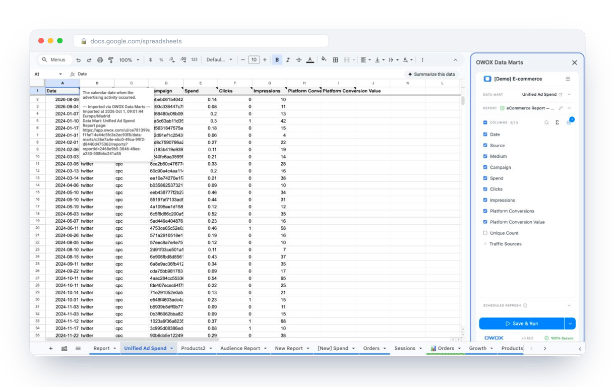
What changes for the person who maintains the sheet:
- Refresh replaces re-export. Refresh current report in the extension menu re-runs the same pull, and a scheduled refresh keeps the tab current without anyone touching it.
- The source is written on the sheet. The header cell of an imported tab carries a note with the data mart it came from, the time of the import and a link to the report.
- No SQL and no warehouse access needed. The analyst decides which data marts and columns are available. You choose from that list.
The extension does not write or change the analyst’s SQL. When the match between two sources is made there once, the sheet receives the columns already side by side, and concatenation goes back to being a formatting task. The extension comes with the OWOX Cloud plans of OWOX Data Marts; spreadsheet reporting describes both ways data reaches a sheet.
Turn your data into decisions.
Governed data marts give you the clean foundation ML needs to actually work.
- No AI hallucinations
- Analyst-governed definitions
- Every number traces to SQL
Frequently Asked Questions
Can CONCATENATE be used inside a QUERY statement?
No. The QUERY language has no concatenation operator, so "select A & B" returns an error. Join the columns before the query, =ARRAYFORMULA(QUERY({A2:A & " " & B2:B, C2:C}, "select Col1 where Col2 > 100", 0)), or join the columns of the result afterwards with TEXTJOIN or the ampersand.
Why does my attempt to concatenate QUERY results return an error?
The usual causes are an ampersand or CONCATENATE written inside the query string, which the query language does not support; a formula with curly braces that is not wrapped in ARRAYFORMULA; column letters used where Col1 and Col2 are required; or typographic quotes pasted from a document.
Can I use QUERY to fetch data from multiple columns and then concatenate them in 1 column?
Yes, you can use QUERY to fetch data from multiple columns and then concatenate them into 1 column. After retrieving the data using QUERY, you can use the & operator or the CONCATENATE function to combine the values from different columns into a single column.
How can I concatenate rows returned by a QUERY function into a single cell?
You can concatenate rows returned by a QUERY function into a single cell with the TEXTJOIN function. First, use QUERY to retrieve the desired rows, then wrap the QUERY function with TEXTJOIN, specifying the delimiter you want to use between each row.