How To Use QUERY And IMPORTRANGE In Google Sheets: With Examples

Importing data from one sheet to another using IMPORTRANGE in Google Sheets is a task that many of us have performed. This article will cover using query and importrange in Google Sheets, but did you know there’s a whole world of possibilities beyond just importing?

With IMPORTRANGE and QUERY functions, you can do much more than that. These functions enable you to transfer all data between Google Sheets, allowing you to manipulate data and gain greater control over what information is nested and displayed in the target spreadsheet. Additionally, you can combine QUERY and IMPORTRANGE to pull data from multiple spreadsheets and perform advanced queries, making them essential tools for effective data management and analysis.

In this article, we’ll explain how to use them, show examples, discuss their benefits, and provide a template that you can use in your work.

Decoding the QUERY Function: Optimized Data Retrieval

The QUERY function in Google Sheets enables you to ask questions and obtain specific answers from your data. This function requires a data source to manipulate information. Let’s explore how it works.

Query Syntax:

=QUERY(data_range,"query_string")

Here is the breakdown:

• This is where you tell the function where to find the information you want to analyze. It could be a range of cells or even an entire sheet.
• query: This is the question you’re asking your data. You write it using special words that the function understands, sort of like giving it instructions.
• [headers]: This part is optional. If your data has headers (such as titles at the top of your columns), you can instruct the function to skip a certain number of rows so it knows where your data begins.

Using QUERY can help avoid the need for complex formulas.

Example:

Let’s say we have a list of students’ names in column B and their scores in column C. To find out who scored higher than 90, you can use the following QUERY formula.

=QUERY(B3:C12, "SELECT B, C WHERE C > 90")

This instructs the function to search cells B3 to C12, identify the names and scores where the score is greater than 90, and display them in the result. So, you’d get a list of students’ names and scores, but only for those who scored 90 or higher.

Understanding IMPORTRANGE Function: Seamless Data Import

The IMPORTRANGE function in Google Sheets helps you bring in data from another sheet or even a different Google Sheets file using the importrange formula.

Syntax of IMPORTRANGE:

=IMPORTRANGE("spreadsheet_url","range_string")

Let’s break it down:

• spreadsheet_url: this is the web address (URL) of the Google Sheets file you want to import data from.
• range_string: it shows which part of the other sheet you want to import. You can think of it as the specific cells or range of cells.

Example:

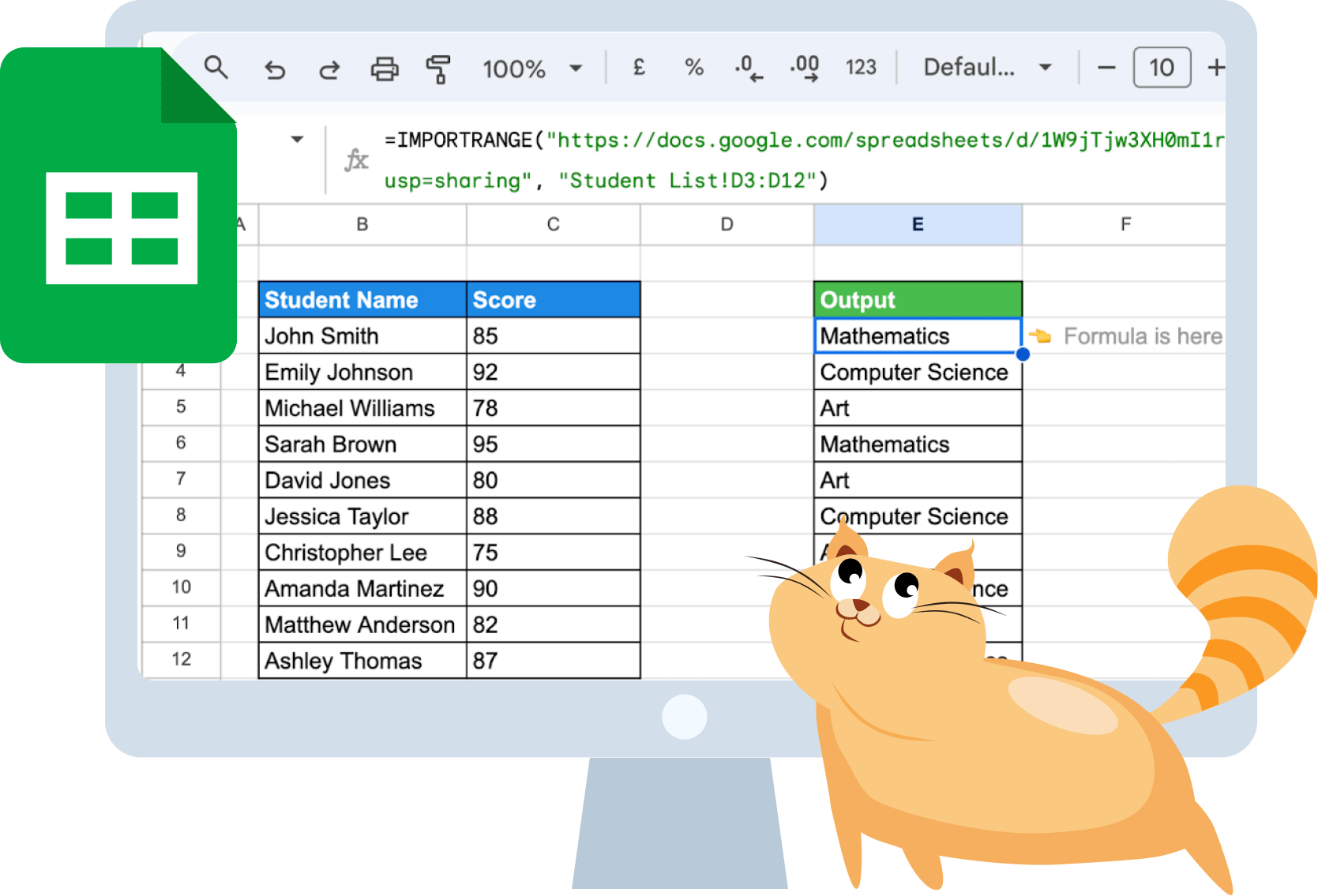
Let’s use our student table from the previous example. Suppose we have a sheet called “Student List” in our Google Sheets file. To import the faculty information for each student from the sheet into our current sheet, we will use the IMPORTRANGE formula, selecting the appropriate imported data range.

=IMPORTRANGE("https://docs.google.com/spreadsheets/d/1W9jTjw3XH0mI1rLVeHXej_vqn1L7dVC1djisb4gJtW4/edit?usp=sharing", "Student List!D3:D12")

This function will import faculty information for each student from the specified range in the “Student List” sheet into our current sheet.

How to Use QUERY And IMPORTRANGE For Advanced Data Manipulation

What if we need to combine data from multiple spreadsheets in Google Sheets and then analyze it in a specific way?

Here’s how it works:

1. Use IMPORTRANGE to fetch data from other sheets or files.
2. Then, wrap the IMPORTRANGE function inside QUERY. This helps you ask questions about the imported data and filter it according to your needs. When filtering data imported from multiple spreadsheets, it's essential to verify that the first column is not empty to ensure that only relevant data is processed in the final output. To use the QUERY function with IMPORTRANGE, wrap the IMPORTRANGE function inside the QUERY function.

QUERY+IMPORTRANGE Syntax in Google Sheets

=QUERY(IMPORTRANGE("spreadsheet_url", "data_range"), "query_string")

• IMPORTRANGE("spreadsheet_url", "data_range") fetches data from another Google Sheets file.
• "spreadsheet_url" is the web address (URL) of the Google Sheets file you want to import data from.
• "data_range" specifies the range of cells from the other sheet that you want to import.
• QUERY() function is wrapped around IMPORTRANGE to filter and manipulate the imported data.
• "query_string" is where you write your query to filter the imported data. You use special keywords and commands to specify what information you want to extract.

QUERY+IMPORTRANGE Example Application

Continuing with our example, let's say we have one sheet with student names and scores, and another with their faculties.

By combining QUERY and IMPORTRANGE, you could find out the faculties of students who scored above 90. For more details, including how to apply multiple criteria, you can refer to the documentation.

Formula:

=QUERY(IMPORTRANGE("https://docs.google.com/spreadsheets/d/1W9jTjw3XH0mI1rLVeHXej_vqn1L7dVC1djisb4gJtW4/edit?usp=sharing", "Student List!B:D"), "SELECT Col1, Col3 WHERE Col2 > 90", 1)

• IMPORTRANGE("https://docs.google.com/spreadsheets/d/ 1W9jTjw3XH0mI1rLVeHXej_vqn1L7dVC1djisb4gJtW4/edit?usp=sharing", "Student List!B:D"): This part imports data from our Google Sheets file, specified by its URL and the range "Student List!B:D". This range covers columns B to D, where column B contains student names, column C contains scores, and column D contains faculties.
• "SELECT Col1, Col3 WHERE Col2 > 90": This is the query string, where:
  • SELECT Col1, Col3: This selects columns 1 (student names) and 3 (faculties) from the imported data.
  • WHERE Col2 > 90: This filters the data to only include rows where the score (in column 2) is greater than 90.
  • 1: This specifies that the first row of the imported data contains headers (student names, scores, faculties), so the QUERY function should skip it.

Discover QUERY and IMPORTRANGE with Our Ready-to-Use Template!

Explore Google Sheets like never before with our template filled with QUERY and IMPORTRANGE formulas. Just download, open, and start analyzing your data!

Get your free template now!

Use Cases Of Combining QUERY And IMPORTRANGE in Google Sheets

With QUERY and IMPORTRANGE in Google Sheets, you can do a lot. You can import specific data, combine data from different sheets, remove unnecessary rows, search for specific text, and more. Handling several spreadsheets is particularly useful when combining and analyzing data, especially in scenarios like business surveys and educational assessments, where similar formats are present across these spreadsheets.

To facilitate this process, you can use the following formula to import and combine data from multiple spreadsheets while adhering to certain criteria.

Mastering these techniques makes your work more efficient. And what’s more, all these cases are available for you in our template.

If you would like to learn more about finding data with specific criteria in Google Sheets, you can read our guide on VLOOKUP functions.

Now, you’re ready to explore the versatility of QUERY and IMPORTRANGE functions further. So let’s dive into each use case and uncover the full potential of combining QUERY with IMPORTRANGE to optimize your data management tasks and Google Sheets experience.

Use Case #1: Importing Specific Data Range

The most basic scenario involves importing a specific data range from another table. Utilising various data sources, including Google Analytics and SEMrush, can provide a comprehensive overview for online marketing purposes. For instance, we have a Google Sheets file with student information, but only want to import the scores and faculties of the students (range B3:C12) into another sheet.

Here's how you can combine IMPORTRANGE with the SELECT clause in QUERY to import specific columns from the "Student List" sheet, and then choose exactly which columns you want to pull.

Formula:

=QUERY(IMPORTRANGE("https://docs.google.com/spreadsheets/d/1W9jTjw3XH0mI1rLVeHXej_vqn1L7dVC1djisb4gJtW4/edit?usp=sharing", "Student List!B:D"), "SELECT Col1, Col2, Col3")

Use Case #2: Merging Multiple Sheets Data

If you have data scattered across different sheets and want to merge it into 1, specifying a source file for each dataset is crucial. QUERY and IMPORTRANGE can help streamline this process. There are two different methods of merging your data.

For merging horizontally, separate IMPORTRANGE functions by commas:

=QUERY({IMPORTRANGE("spreadsheet1_url", "data_range"), IMPORTRANGE("spreadsheet2_url", "data_range"),..}, "query_string")

For merging vertically, separate IMPORTRANGE functions by semicolons:

=QUERY({IMPORTRANGE("spreadsheet1_url"; "data_range"), IMPORTRANGE("spreadsheet2_url"; "data_range"),..}, "query_string")

Remember to import separately from each sheet before using QUERY and IMPORTRANGE, especially when applying the where clause to avoid errors. Specify the source, such as 'Orders from Airtable', to ensure accurate data import.

We have scores in another sheet named “Scores” and faculties in named “Faculty”. To merge this information into 1 sheet using QUERY and IMPORTRANGE, use the formula below.

Formula:

=QUERY({IMPORTRANGE("https://docs.google.com/spreadsheets/d/1oad79FkDOx2iGdeiJDEcKeBcVZGDHDl9MDiK0WAa13g/edit?usp=sharing", "Scores!B2:C12"), IMPORTRANGE("https://docs.google.com/spreadsheets/d/1oad79FkDOx2iGdeiJDEcKeBcVZGDHDl9MDiK0WAa13g/edit?usp=sharing", "Faculty!B2:C12")}, "SELECT Col1, Col2, Col4")

Note that when you import data using IMPORTRANGE from a specific spreadsheet for the first time, the formula prompts you to grant access. Simply click on the small button that appears in the cell to allow access.

Use Case #3: Eliminating Extra Rows in Imported Data

You can use the “limit” and “offset” QUERY clauses to control the number of rows imported and remove unnecessary ones.

The “limit” clause sets the maximum number of rows to import, excluding the header. For instance, “limit 5” would import only 5 rows of data.

Meanwhile, the “offset” clause determines the number of rows to skip from the top of the imported data. For example, “offset 2” would skip the first 2 rows of data.

So, if you use “limit 5” and “offset 2” together, you’ll import 5 rows of data starting from the third row. This helps streamline your data analysis by focusing only on the relevant information.

Efficiently managing numerical data, such as total price, is crucial during data manipulation processes. This ensures that you can apply conditions to focus on products with a total price exceeding a certain amount when transferring data from Airtable.

Formula:

=QUERY(IMPORTRANGE("https://docs.google.com/spreadsheets/d/1W9jTjw3XH0mI1rLVeHXej_vqn1L7dVC1djisb4gJtW4/edit?usp=sharing", "Student List!B:D"), "SELECT Col1, Col2, Col3 LIMIT 5 OFFSET 2")

Use Case #4: Renaming Imported Columns

You can customize the imported column names using the “label“ QUERY clause.

The “label” clause allows you to rename the headers of the imported columns. For instance, we can change “Score” to “Grade”.

Additionally, you can use the SELECT SUM function to filter and aggregate data, such as calculating the total GDP for specified regions, which is useful for generating informative dashboards and reports.

To achieve this task:

• Import columns B, C, and D from the “Student List” spreadsheet.
• Limit the imported rows to 5, excluding the header row.
• Rename the headers of the imported columns, replacing “Score” with “Grade”.

Formula:

=QUERY(IMPORTRANGE("https://docs.google.com/spreadsheets/d/1W9jTjw3XH0mI1rLVeHXej_vqn1L7dVC1djisb4gJtW4/edit?usp=sharing", "Student List!B:D"), "SELECT Col1, Col2, Col3 LIMIT 5 LABEL Col2 'Grade'")

This formula imports the first 5 rows of data from columns B, C, and D of the "Student List" sheet and renames the header accordingly.

Make sense of your data

Automatically generate Pivots & Charts in Google Sheets!

Visualize Your Data

Use Case #5: Adjusting Imported Columns Values

In case you need to apply custom formatting to the values in imported columns, you can adjust the formatting of imported columns using the “format” QUERY clause. Advanced users often utilize the query importrange in Google Sheets to manipulate imported datasets effectively, showcasing their skills and enhancing their understanding of these functions.

For instance, you can format dates in the "E" column to display only the month and year.

For this:

• Import columns B, C, D, and E from the "Student List" spreadsheet.
• Format the values in the "E" column to display only the month and year.

Formula:

=QUERY(IMPORTRANGE("https://docs.google.com/spreadsheets/d/1W9jTjw3XH0mI1rLVeHXej_vqn1L7dVC1djisb4gJtW4/edit?usp=sharing","Student List!B:E"), "SELECT Col1,Col2,Col3,Col4 FORMAT Col4 'mmm-yyyy'")

Use Case #6: Filtering Imported Data

With the QUERY clause in Google Sheets, you can selectively filter rows within imported columns by applying specific conditions using the WHERE statement. By combining functions like QUERY and IMPORTRANGE, you can pull specific data from various sources into one spreadsheet, enabling better organization and analysis of information across multiple sheets.

Let's say, we need to apply a filter to the imported data, specifying that only rows where the value in column C is greater than or equal to 80 should be included.

Formula:

=QUERY(IMPORTRANGE("https://docs.google.com/spreadsheets/d/1W9jTjw3XH0mI1rLVeHXej_vqn1L7dVC1djisb4gJtW4/edit?usp=sharing","Student List!B:E"), "SELECT Col1,Col2,Col3,Col4 WHERE Col2>=80")

Use Case #7: Applying Multiple Criteria for QUERY and IMPORTRANGE

When using the WHERE statement with QUERY and IMPORTRANGE, you're not limited to just 1 rule, and can actually add a few rules using AND or OR.

So, let's change our previous formula a bit. Along with getting students who scored 80 or more in column C, let's also get students whose names start with the letter "J".

Formula:

=QUERY(IMPORTRANGE("https://docs.google.com/spreadsheets/d/1W9jTjw3XH0mI1rLVeHXej_vqn1L7dVC1djisb4gJtW4/edit?usp=sharing","Student List!B:E"), "SELECT Col1,Col2,Col3,Col4 WHERE Col1 STARTS WITH 'J' AND Col2>=80")

Use Case #8: Searching for Specific Text Within Imported Data

We can specify criteria for what a particular column should contain to meet our needs. This can be done using the WHERE clause with a contains operator.

Let's use the formula below to filter our student data only to retrieve those in the "Mathematics" faculty.

Formula:

=QUERY(IMPORTRANGE("https://docs.google.com/spreadsheets/d/1W9jTjw3XH0mI1rLVeHXej_vqn1L7dVC1djisb4gJtW4/edit?usp=sharing","Student List!B:E"), "SELECT Col1,Col2,Col3,Col4 WHERE Col3 CONTAINS 'Mathematics'")

Use Case #9: Sorting Imported Data

When we're using the ORDER BY clause with QUERY, we can sort our data based on a specific column, either in ascending or descending order.

In this case, we want to:

1. Import columns B, C, D, and E from the spreadsheet.
2. Filter the imported data so that only values in column B greater than or equal to 80 are included.
3. Sort the imported data by the date of birth (column E) in descending order.

Formula:

=QUERY(IMPORTRANGE("https://docs.google.com/spreadsheets/d/1W9jTjw3XH0mI1rLVeHXej_vqn1L7dVC1djisb4gJtW4/edit?usp=sharing","Student List!B:E"), "SELECT Col1,Col2,Col3,Col4 WHERE Col2>=80 ORDER BY Col4 DESC")

Use Case #10: Arithmetic Calculations on Imported Data

We can perform basic arithmetic operations like add (+), subtract (-), multiply (*), and divide (/) columns imported from a spreadsheet and display the result as a separate column.

Our task is to:

• Get the student names along with their scores from 2 specific columns (D and F) in the 'Student List all scores' spreadsheet.
• Add up these scores for each student and show the total as a new column named 'Scores Total'.

Formula:

=QUERY(IMPORTRANGE("https://docs.google.com/spreadsheets/d/1W9jTjw3XH0mI1rLVeHXej_vqn1L7dVC1djisb4gJtW4/edit?usp=sharing", "Student List!B:E"), "SELECT D, SUM(C) WHERE D <> '' GROUP BY D LABEL D 'Faculty', SUM(C) 'Total Scores'")

Use Case #11: Aggregating Imported Data

In Google Sheets, you can use aggregation functions within select, order by, label, and format QUERY clauses to perform calculations on imported columns:

• avg() calculates the average of all numbers in a column.
• sum() calculates the total sum of all numbers in a column.
• count() calculates the total quantity of items in a column (excluding rows with empty cells).
• max() identifies the maximum value in a column.
• min() identifies the minimum value in a column.

Our task:

1. Summarize the scores (column C) for each faculty (column D), specifically Mathematics, Computer Science, and Art.
2. Display the total scores for each faculty in a new column named 'Total Scores'.

Formula:

=QUERY(IMPORTRANGE("https://docs.google.com/spreadsheets/d/1W9jTjw3XH0mI1rLVeHXej_vqn1L7dVC1djisb4gJtW4/edit?usp=sharing", "Student List!B:E"), "SELECT D, SUM(C) WHERE D <> '' GROUP BY D LABEL D 'Faculty', SUM(C) 'Total Scores'")

Use Case #12: Executing Scalar Functions on Imported Data

When using scalar functions, we can transform imported data into a single value.

Consider the table with columns B to E containing student names, scores, faculty, and date of birth. If you apply the year() function to the date of birth values, it will extract the year. So, if you have dates like 26/01/1994, year() will return 1994.

Formula:

=QUERY(IMPORTRANGE("https://docs.google.com/spreadsheets/d/1W9jTjw3XH0mI1rLVeHXej_vqn1L7dVC1djisb4gJtW4/edit?usp=sharing", "Student List!B:E"), "SELECT Col1, Col2, Col3, YEAR(Col4) LABEL YEAR(Col4) 'Year of Birth'")

Troubleshooting Common Issues with QUERY and IMPORTRANGE

When using QUERY and IMPORTRANGE in Google Sheets, you may encounter some common issues. Here are a few tips to help you troubleshoot and avoid potential errors:

• Check for typos or incorrect syntax: Ensure that your QUERY formula is free of typos and follows the correct syntax. Even a small mistake can cause the formula to fail.
• Verify referenced columns: Ensure that all referenced columns are present in the imported data. If a column is missing or incorrectly referenced, the QUERY function will not work as expected.
• Double-check the IMPORTRANGE function: Ensure that the spreadsheet URL and range specified in the IMPORTRANGE function are correct. An incorrect URL or data range can lead to errors during data import.
• Verify permissions: Make sure you have the necessary permissions to access the source spreadsheet. If you don’t have access, the IMPORTRANGE function will not be able to import the data.

By keeping these tips in mind, you can effectively troubleshoot and resolve common issues when using the QUERY and IMPORTRANGE formula in Google Sheets. For more detailed solutions, you can refer to our articles on IMPORTRANGE and QUERY error solutions.

Sharpen Your Knowledge with These Google Sheets Guides

If you want to improve your Google Sheets skills, learn more about mastering more advanced functions like ARRAY, XLOOKUP, and UNIQUE:

• XLOOKUP: Helps find and retrieve information from your spreadsheet quickly and easily.
• ARRAY: Conducts calculations across multiple cells or ranges, delivering multiple results simultaneously.
• UNIQUE: Extracts values from a range and removes any duplicates.
• Pivot Table: This adaptable tool simplifies the summarization, organization, and examination of extensive data sets, allowing for easy extraction of insights and identification of trends.
• CONCATENATE Function: This function combines multiple text items into a single continuous string, providing a seamless way to merge text from different cells.
• IMPORT Function: Fetches and parses data from structured XML files via URLs, enabling direct display in your sheets.

Advancing Your Analytics Journey with OWOX: Reports, Charts & Pivots

OWOX: Reports, Charts & Pivots Extension offers a more straightforward way to work with data, even if you're not a spreadsheet expert. With its intuitive interface, you can work with complex data and produce high-quality reports. Whether you're analyzing sales, customer behavior, or marketing data, the OWOX Reports Extension for Google Sheets helps you extract useful data without the need to master complex spreadsheet techniques.