How to Use the QUARTILE Function in Google Sheets for Data Analysis

Working with data can be overwhelming, but the right tools make it much easier. Google Sheets provides powerful functions like QUARTILE to help you analyze and interpret data effectively. This function allows you to divide data into quartiles, giving you a clearer view of its distribution and spread.

Whether you’re identifying trends, spotting outliers, or segmenting information, the QUARTILE function turns raw data into meaningful insights.

In this article, we’ll walk you through how to use the QUARTILE function for data analysis, complete with practical examples and best practices. Let’s dive in and see how you can unlock smarter data-driven decisions with Google Sheets!

The Purpose of the QUARTILE Function in Google Sheets

The QUARTILE function in Google Sheets helps divide a dataset into four equal parts, providing valuable insights into its distribution. By identifying the minimum, maximum, and three key quartile values, this function allows you to analyze how data is spread across a range. 

It’s particularly useful for comparing datasets, detecting patterns, and spotting outliers. For example, you can use the first and third quartiles to calculate the interquartile range (IQR), which highlights the central 50% of your data and helps identify unusual values. 

Whether you’re analyzing sales performance, test scores, or customer behavior, the QUARTILE function offers a simple yet effective way to interpret data and make more informed decisions.

Understanding the QUARTILE Function: Syntax and Examples

The QUARTILE function in Google Sheets helps you understand how data is distributed by dividing it into four equal parts. It’s useful for analyzing data spread, identifying trends, and spotting patterns. By using quartile values, you can gain deeper insights into your data and make more informed decisions.

QUARTILE

The QUARTILE function in Google Sheets divides a dataset into four equal parts, or quartiles, to help analyze data distribution. It returns values corresponding to the first, second (median), third, and fourth quartiles. This function is useful for identifying data spread, understanding trends, and spotting outliers.

Syntax of QUARTILE

The syntax of the QUARTILE function in Google Sheets is:

=QUARTILE(data, quartile_number)

Let’s break down what these parameters represent:

• data: The array or range containing the dataset to analyze.
• quartile_number: Specifies which quartile value to return:
  
  • 0: Returns the minimum value (0% mark).
  • 1: Returns the first quartile value (25% mark).
  • 2: Returns the median (50% mark).
  • 3: Returns the third quartile value (75% mark).
  • 4: Returns the maximum value (100% mark).

This function helps identify data spread and quartile values, useful for understanding distribution patterns.

Example of QUARTILE

Now, using the monthly sales data, we will calculate the 1st quartile to determine the sales figure below which the bottom 25% of reps fall.

Formula Explanation:

=QUARTILE(C3:C12, 1)

• C3:C12: Refers to the range containing the sales data for all 10 products.
• 1: Indicates that you want to calculate the 1st quartile (25% mark).

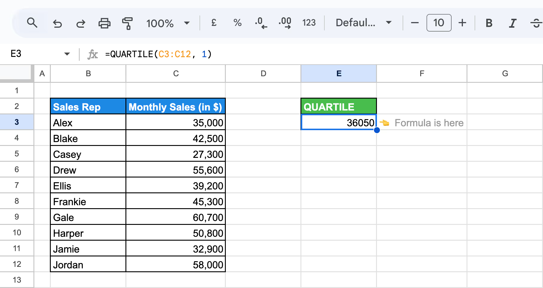
In cell E3, the formula will return the sales figure representing the 1st quartile. This lets you identify which products are in the bottom 25% of sales performance.

QUARTILE.INC

In Google Sheets, QUARTILE and QUARTILE.INC work the same way, calculating quartiles, including the data’s boundaries. QUARTILE.INC ensures compatibility with older sheets while offering consistency with modern function names, avoiding confusion for users familiar with the original QUARTILE function.

QUARTILE.EXC

The QUARTILE.EXC function in Google Sheets calculates quartiles while excluding the dataset's boundary values. It returns the first, second, or third quartile, ignoring the minimum and maximum values. This function provides a refined view of the dataset’s distribution by focusing on the internal range of data.

Syntax of QUARTILE.EXC

The syntax of the QUARTILE.EXC function in Google Sheets is:

=QUARTILE.EXC(data, quartile_number)

Let’s break down what these parameters represent:

• data: The array or range containing the dataset to analyze.
• quartile_number: Specifies which quartile value to return:
  
  • 1: Returns the value closest to the first quartile (25% mark), excluding boundary values.
  • 2: Returns the value closest to the median (50% mark), excluding boundary values.
  • 3: Returns the value closest to the third quartile (75% mark), excluding boundary values.

This function excludes the extreme minimum and maximum values from the quartile calculations.

Example of QUARTILE.EXC

Let’s say you’re analyzing monthly sales performance data and want to find the 1st quartile, excluding extreme values, to pinpoint lower-performing reps in the dataset.

Formula Explanation:

To calculate the 1st quartile (25% mark) excluding boundary values, use the following formula:

=QUARTILE.EXC(C3:C12, 1)

• C3:C12: Refers to the range containing sales data.
• 1: Specifies the quartile you want to calculate by using the QUARTILE.EXC function

In E3, QUARTILE.EXC function, the formula will return a value of around 34475.

Master the QUARTILE Function with Our Template!

All the examples from the article are ready for you in this preloaded template. Download it now and start analyzing data with the QUARTILE function in Google Sheets effortlessly.

Get You Free Template Now!

Detailed Examples of Applying the QUARTILE Function

The QUARTILE function in Google Sheets helps divide a dataset into four equal parts, allowing users to understand the distribution of values. By applying it, businesses can analyze performance metrics, identify data spread, and detect outliers for more informed decision-making.

Finding All Quartiles Using QUARTILE.INC Function

The QUARTILE.INC function in Google Sheets allows you to calculate all quartiles within a dataset, helping you divide the data into four equal parts. This function is particularly useful for analyzing data distribution and identifying key performance segments, such as top or bottom quartiles.

Example of all Quartiles Using QUARTILE.INC

With the same monthly sales figures, you want to divide the sales data into four equal segments to understand performance distribution.

Formula explanation:

To calculate each quartile, use the following formulas in different cells:

Minimum (0th quartile):

=QUARTILE(C3:C10, 0)

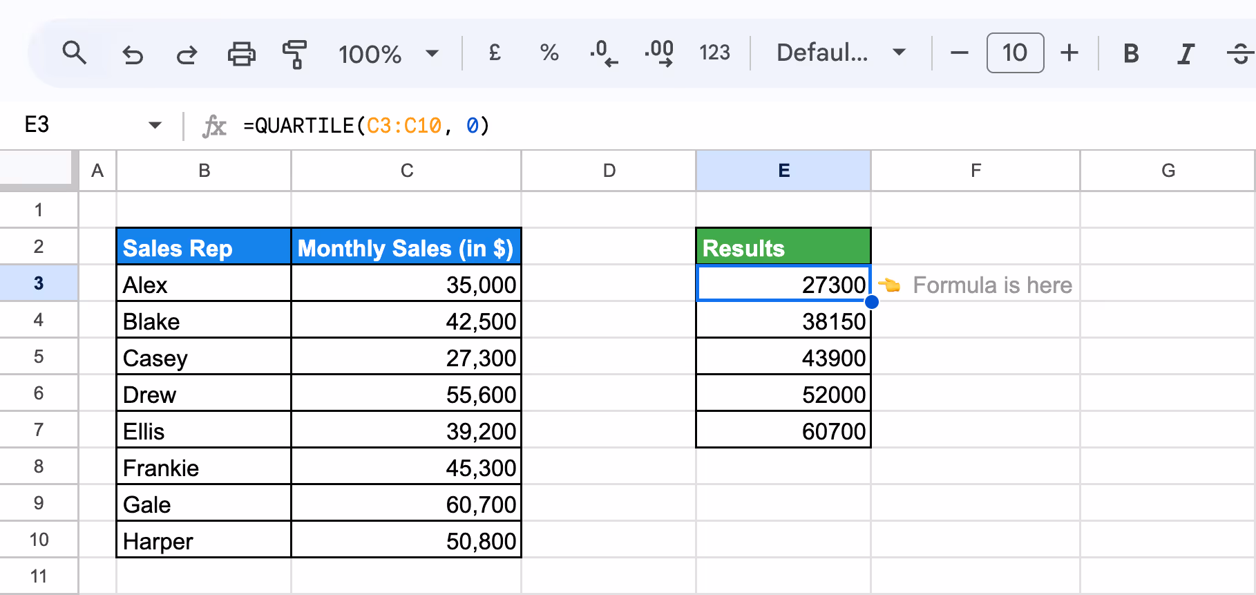
First quartile (25th percentile):

=QUARTILE(C3:C10, 1)

Median (50th percentile):

=QUARTILE(C3:C10, 2)

Third quartile (75th percentile):

=QUARTILE(C3:C10, 3)

Maximum (100th percentile):

=QUARTILE(C3:C10, 4)

• C3:C7: Refers to the range containing your sales data.
• 0 to 4: Refers to the quartile number (0 for minimum, 4 for maximum).

The QUARTILE.INC function provides a clear breakdown of your team's sales data, helping you quickly identify performance tiers.

Calculating the Median (Second Quartile) with QUARTILE.EXC

The QUARTILE.EXC function in Google Sheets helps calculate the median, or second quartile, which divides the dataset into two halves. It’s useful for determining the midpoint in data, helping businesses assess performance metrics like response times or sales figures.

Let’s use the dataset of monthly sales figures again. You want to find the second quartile (the median) to assess the team's overall performance.

To calculate the median sales figure, use the following formula:

Formula explanation:

=QUARTILE.EXC(C3:C12, 2)

• B2:B11: Refers to the range containing monthly sales data for all 10 sales reps.
• 2: Represents the second quartile (the median).

The formula will return the median sales figure. For instance, if the result is $43,900, it indicates that half of the sales reps have monthly sales below $43,900, and the other half have sales above this amount.

Using QUARTILE.INC with an Array of Numbers and a Range of Cells

The QUARTILE.INC function calculates quartiles for both arrays and cell ranges, helping to analyze data distribution and trends efficiently.

QUARTILE.INC with an array of numbers

Let’s use an array of sales figures to calculate the second quartile (median) using the QUARTILE.INC function. This helps determine the midpoint of the sales data, providing insights into overall performance.

Formula explanation:

=QUARTILE.INC({35000, 42500, 27300, 55600, 39200, 45300, 60700, 50800, 32900, 58000}, 2)

• {35000, 42500, 27300, 55600, 39200, 45300}: This array represents the sales figures for all 6 sales reps.
• 2: Specifies the quartile you want to calculate; 2 represents the second quartile (or the median).

This formula will return $40850, which is the median (second quartile) of the array.

Using QUARTILE.INC with a range of cells

Let’s use the same dataset of sales figures, but input it into a range of cells in Google Sheets to calculate the second quartile (median) using the QUARTILE.INC function.

Formula explanation:

=QUARTILE.INC(C13:C18, 2)

• C13:C18: Refers to the range of cells containing the sales figures.
• 2: Indicates that you want to calculate the second quartile (the median).

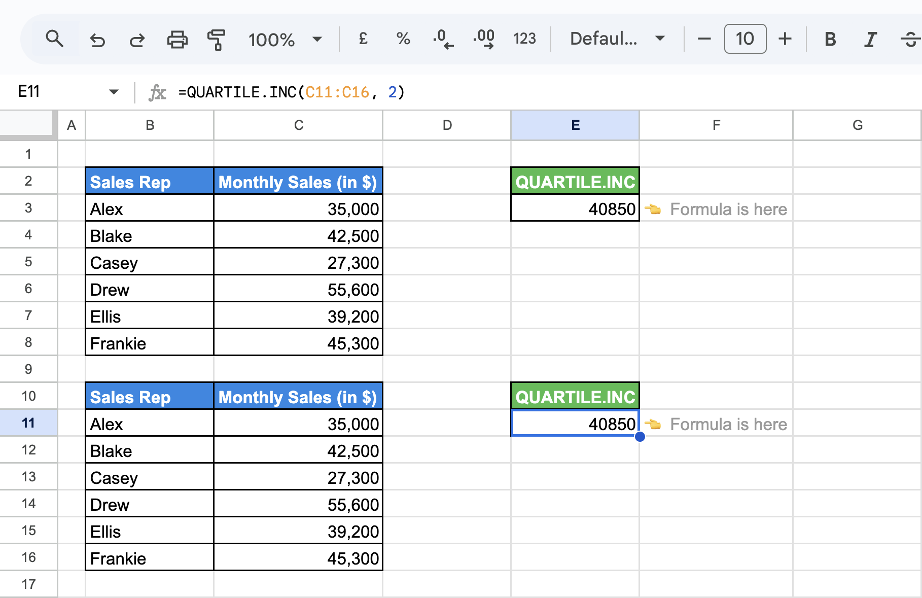
The formula will return 40850, which is the median (second quartile) of the sales figures in the range.

Using arrays with QUARTILE.INC involves entering data directly into the formula, ideal for small, static datasets. 

In contrast, using a range of cells references cell ranges, making it better for larger or frequently updated datasets, as changes in cells automatically update the formula’s result.

Combining the QUARTILE Function with Other Functions in Google Sheets

Combining the QUARTILE function with other functions in Google Sheets can enhance your data analysis. Pair it with IF, AVERAGE, or COUNTIFS to create more dynamic and insightful reports. This approach helps you filter data, calculate averages for specific quartile ranges, and identify patterns or outliers for deeper analysis and better decision-making.

Using PERCENTILE and QUARTILE with the IF Function

The IF function in Google Sheets allows you to apply logical conditions to your data. It can categorize or filter data based on specific thresholds when combined with the PERCENTILE and QUARTILE functions. This can be useful for analyzing performance, identifying outliers, or segmenting data.

Example of PERCENTILE with IF

In this example, you want to determine a specific region's 75th percentile of sales (e.g., "North"). You will use the PERCENTILE function combined with IF to filter the data dynamically based on the region selected.

Formula Explanation:

=ArrayFormula(PERCENTILE(IF($B$3:$B$11=$G4, $D$3:$D$11), 0.75))

• $B$3:$B$11: This range contains the region data (North, South, East).
• $G4: This is where you input the region you want to calculate the percentile for (e.g., "North").
• $D$3:$D$11: This range contains the corresponding sales data for each sales rep.
• 0.75: This calculates the 75th percentile (top 25%).

Here, the formula is used with ARRAYFORMULA because the IF statement returns an array of values.

Example of QUARTILE with IF

Now, you want to focus on high sales figures, specifically those between $30,000 and $55,000, and identify the top 25% of sales (3rd quartile) within this range for further analysis.

Formula Explanation:

=ArrayFormula(QUARTILE(IF((C3:C11>=30000)*(C3:C11<=55000), C3:C11), 3))

• C3: This range contains the sales data for each year.
• (C3:C11>=30000)*(C3:C11<=55000): This condition filters the sales data to include only those sales figures that are between $30,000 and $55,000, inclusive. It returns TRUE for sales within this range and FALSE otherwise.
• IF(..., B2:B10): This part of the formula returns only the sales values that meet the specified condition.
• QUARTILE(..., 3): Calculates the 3rd quartile (75th percentile) of the filtered sales data, showing the point where the top 25% of the selected sales range lies.

Here, the formula is used with ARRAYFORMULA since the IF statement returns an array of values. Using this formula, the result will show the 3rd quartile value of $44,600.

Resolving Common Issues with the QUARTILE Function in Google Sheets

When using the QUARTILE function in Google Sheets, you may encounter common issues such as errors or unexpected results. These often arise from non-numeric values, empty datasets, or incorrect range references. To avoid problems, ensure your data is clean, the range is correctly defined, and all values are properly formatted for accurate results.

#NUM! Error

⚠️ Error: The #NUM! error in QUARTILE.EXC occurs when the quartile value is outside the valid range of 0 to 4. This prevents the function from calculating the desired quartile accurately.

✅ Solution: Ensure the quartile value in QUARTILE.EXC is within the correct range (0 to 4). Double-check your inputs and adjust the formula to use valid numeric values for accurate results.

#N/A Error

⚠️ Error: The #N/A error in QUARTILE.EXC occurs when the dataset is empty, contains non-numeric values (like text), or the quartile value you’re calculating is not found within the dataset.

✅ Solution: Ensure the dataset is not empty and contains only numeric values. Remove any non-numeric entries and verify that the specified quartile exists within the data range. Double-check your inputs to avoid errors.

#DIV/0! Error

⚠️ Error: The #DIV/0! error in QUARTILE.EXC occurs when the dataset is empty, contains no numeric values, or when the quartile value is invalid (e.g., less than 0 or greater than 4).

✅ Solution: Ensure the dataset contains valid numeric values and is not empty. Verify that the quartile value is within the correct range (0 to 4). Clean your data and check the formula parameters to avoid this error.

Invalid Range

⚠️ Error: The Invalid Range error in QUARTILE.EXC occurs when the provided range is empty, contains non-numeric values, or is incorrectly referenced. This prevents the function from calculating the quartile accurately.

✅ Solution: Ensure the data range is not empty and contains only numeric values. Remove non-numeric entries and verify that the range is correctly referenced. Double-check your formula to ensure the data range is properly defined.

Omitting Value Parameter

⚠️ Error: The Omitting Value Parameter error in QUARTILE.EXC occurs when a required parameter, such as the data range or quartile value, is missing. This prevents the function from calculating the quartile correctly.

✅ Solution: Ensure the function includes all necessary parameters, such as the data range and a valid quartile value (0 to 4). Double-check the formula to ensure no arguments are missing or left blank.

Best Practices for Effectively Using the QUARTILE Function in Google Sheets

For effective use of the QUARTILE function in Google Sheets, start with well-organized data and verify your inputs. Ensure your range contains only relevant values, and select a valid quartile. Reviewing and cross-checking your results can help improve accuracy and provide deeper insights into your data distribution.

Ensure Data Accuracy and Organization

Ensure data accuracy and organization when using the QUARTILE function in Google Sheets for reliable results. Clean your dataset by removing non-numeric values and empty cells. Verify that your data range is correctly defined and complete. Well-organized data reduces errors, improves calculation accuracy, and provides clearer insights into data distribution and patterns.

Understand the Context of Your Data

Understanding the context of your data is essential when using the QUARTILE function in Google Sheets. Consider the data’s distribution, scale, and purpose before analyzing quartiles. Knowing how your data relates to real-world scenarios helps you interpret quartile results accurately and make more informed decisions based on your findings.

Combine with Other Functions for Deeper Insights

Combine the QUARTILE function with other functions like AVERAGE, IF, or COUNTIFS for deeper insights into your data. This approach helps you filter and group data more effectively, identify patterns, and calculate averages within specific quartile ranges, providing a clearer picture of data distribution and trends.

Use Conditional Formatting for Better Visualization

Use conditional formatting with the QUARTILE function in Google Sheets to visualize data more effectively. Apply color scales or custom rules to highlight specific quartile ranges, making it easier to spot trends, detect outliers, and identify patterns at a glance for more informed decision-making.

Experiment with Different Data Ranges

Experimenting with different data ranges when using the QUARTILE function can reveal new insights. Analyze subsets of your data, such as specific time periods or categories, to better understand data distribution. This approach helps identify patterns, detect anomalies, and compare quartile results across various data segments for more targeted analysis

Verify Your Results with Cross-Checks

Verifying your results with alternative methods or visual tools like charts and graphs is essential for accuracy. Cross-checking calculations ensures data reliability, helping you detect inconsistencies or errors before making informed decisions. This approach improves the quality of your analysis and enhances data-driven decision-making.

Powerful Google Sheets Functions for Enhanced Data Analysis

Learn the full power of Google Sheets, with essential functions tailored for comprehensive data analysis. These advanced formulas simplify complex tasks, enabling you to handle large datasets, automate processes, and extract valuable insights effortlessly.

• SUM, SUMIF, and SUMIFS: Adds values from a range, with SUMIF and SUMIFS allowing conditional summing based on one or multiple criteria, simplifying targeted calculations.
• UNIQUE: Removes duplicates, providing a list of distinct values for cleaner analysis and identifying unique data points.
• PIVOT: Automatically summarizes data with pivot tables, helping you report, organize, and visualize trends effortlessly.
• IMPORTRANGE: Imports data from external Google Sheets, consolidating multiple sources into one, streamlining your data analysis.
• MATCH: Finds the position of a value within a range, useful for dynamic lookups when combined with other functions like INDEX.
• COUNTA: Counts non-empty cells in a range, giving a quick overview of your dataset’s size and density.
• MAX, MIN, MEDIAN: Returns the highest, lowest, and middle values in a dataset, providing insights into data distribution and central tendency.
• AVERAGE: Calculates the mean of a set of numbers, highlighting central trends and performance averages in your data.

Effortlessly Analyze Your Data with OWOX: Reports, Charts, and Pivot Tables

OWOX makes data analysis effortless by transforming complex data into actionable insights. OWOX Reports helps you visualize trends, identify patterns, and make data-driven decisions. Managing large datasets becomes seamless, allowing you to find key insights quickly.

Customizable reports and filters let you focus on the metrics that matter most to your business. Its intuitive interface enhances efficiency, saving time while ensuring accurate and reliable data analysis.