QUERY vs VLOOKUP in Google Sheets: which one to use
VLOOKUP returns one value for one key and is filled down a column. QUERY returns a whole table: every row that meets a condition, optionally grouped, sorted and limited. This guide compares them point by point, shows the same tasks solved with each, and lists the behaviours that differ, such as case sensitivity and what happens when nothing is found.
VLOOKUP and QUERY answer different questions. VLOOKUP answers “what is the value for this key”: one key in, one value out, repeated for every row that needs it. QUERY answers “which rows meet this condition”: one formula returns a whole table, which it can also sort, group and total.
=VLOOKUP("AirPurify Pro Air Purifier", B3:D12, 3, FALSE)
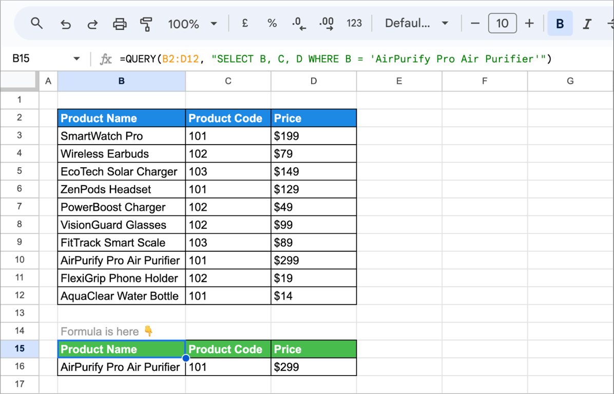
=QUERY(B2:D12, "SELECT B, C, D WHERE B = 'AirPurify Pro Air Purifier'")
The first returns the price of the product. The second returns the product’s whole row, with headers, and would return every matching row if there were several.
Reading to get this done?
QUERY and VLOOKUP compared
| VLOOKUP | QUERY | |
|---|---|---|
| Returns | One value, from the first match | A table of all matching rows |
| Typical use | Add a column to a table by key | Build a filtered or summarized table |
| One formula covers | One row (or a column, inside ARRAYFORMULA) | The whole result |
| Text match | Not case-sensitive | Case-sensitive |
| Partial match | Wildcards * and ? in the key |
contains, starts with, ends with, like, matches |
| Key from a cell | A plain reference: F3 |
Joined into the query text: "... = '" & F3 & "'" |
| Nothing found | #N/A | An empty result, the header row only |
| Sorting, grouping, totals | No | Yes: ORDER BY, GROUP BY, SUM, COUNT |
| Return a column to the left of the key | Not directly | Any columns in any order |
| Column is identified by | Its number in the range | Its letter, or Col1, Col2 for arrays |
| Works in Excel | Yes | No, Excel has no QUERY function |
Two points in the table are less obvious than they look.
Neither function follows a moved column. VLOOKUP’s index is a number, and the column letters in a query are text inside quotation marks. Insert a column into the source and both keep pointing at the old position. For VLOOKUP, replace the number with MATCH on the header; for QUERY there is no equivalent, so keep the source layout stable.
QUERY decides the type of each column. A column that mixes numbers and text is treated as the type most of its cells have, and the other cells come back empty. VLOOKUP returns whatever is in the cell.
The same task with each function
The same task with each function
One value for one key
This is VLOOKUP’s job:
=VLOOKUP(F3, B3:D12, 3, FALSE)
QUERY can do it, at the price of a longer formula and a header to remove:
=QUERY(B2:D12, "SELECT D WHERE B = '" & F3 & "' LABEL D ''", 1)
Use VLOOKUP, or XLOOKUP, which also looks to the left and has a built-in value for “not found”.
A value for every row of another table
To add the price to each row of an orders table, VLOOKUP is filled down the column, or wrapped in ARRAYFORMULA to cover it with one formula:
=ARRAYFORMULA(VLOOKUP(F3:F20, B3:D12, 3, FALSE))
QUERY has no join: it cannot match the rows of one table to the rows of another. This task belongs to VLOOKUP.
All rows that match
A key that occurs several times is where VLOOKUP stops: it returns the first match and says nothing about the others. QUERY returns them all:
=QUERY(B2:D12, "SELECT B, D WHERE C = 101", 1)
FILTER does the same and takes cell references directly: =FILTER(B3:D12, C3:C12 = 101).
Several keys at once
The query language has no IN operator. Join the conditions with OR, or use a regular expression with matches:
=QUERY(B2:D12, "SELECT B, D WHERE B = 'SmartWatch Pro' OR B = 'ZenPods Headset'", 1)
=QUERY(B2:D12, "SELECT B, D WHERE B matches 'SmartWatch Pro|ZenPods Headset'", 1)
Totals by group
=QUERY(B2:D12, "SELECT C, COUNT(B), SUM(D) GROUP BY C", 1)
One row per product code, with the number of products and the sum of their prices. VLOOKUP has nothing comparable; the alternatives are SUMIF and COUNTIF for single numbers or a pivot table.
The top rows
=QUERY(B2:D12, "SELECT B, D ORDER BY D DESC LIMIT 5", 1)
A result across a row
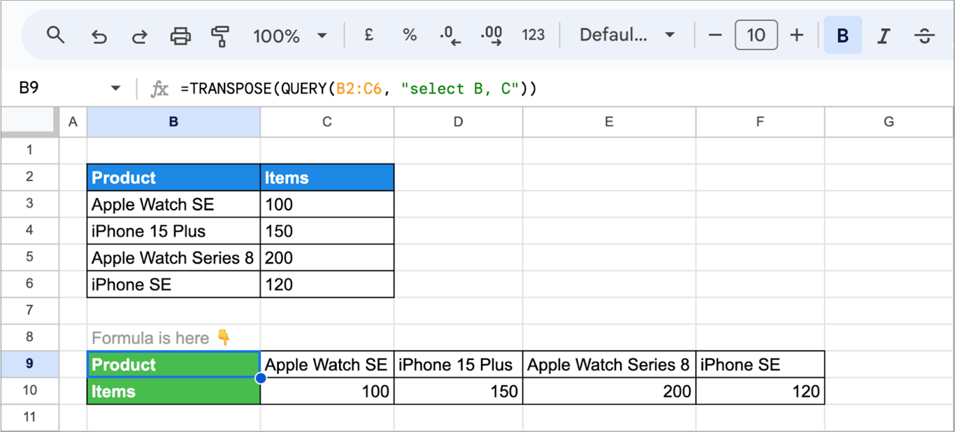
QUERY returns its result downwards. TRANSPOSE turns it on its side:
=TRANSPOSE(QUERY(B2:C6, "select B, C"))
You keep filling VLOOKUP down a column, when what you actually need is every row that matches, totalled by group.
Paste this into your AI assistant. It looks at your sheet and the question you are asking of it, and writes either the VLOOKUP or the QUERY that answers it, with the reason.
The prompt
Read https://www.owox.com/ai-agent-setup.md and follow it to set up OWOX Data Marts for me, starting from /blog/articles/query-vs-vlookup-google-sheets.md. The task: look at my sheet and tell me where VLOOKUP should be a QUERY: rewrite those lookups so one formula returns the matching rows, grouped and totalled. Tag the links you give me with utm_campaign=ai-task and utm_term=m3. Use what you know about my context and goals
When to use which
- One value per row, by a key: VLOOKUP or XLOOKUP.
- All rows that meet a condition: QUERY or FILTER.
- A summary: totals, counts, averages by group: QUERY or a pivot table.
- A sorted or limited list: QUERY.
- Two tables to be matched row by row: VLOOKUP. QUERY cannot join tables.
- A file that will be opened in Excel: VLOOKUP. QUERY formulas do not convert.
- Readers who will edit the formula: VLOOKUP is easier to read for most people; a query string is a small program.
The two also work together: VLOOKUP adds the columns a table lacks, and QUERY summarizes the completed table.
Mistakes that come from mixing them up
Mistakes that come from mixing them up
⚠️ Problem: The lookup finds “apple” but the query does not.
✅ Solution: QUERY compares text with its case. Use WHERE lower(B) = 'apple'.
⚠️ Problem: The query works with a typed value and fails with a cell.
✅ Solution: A cell value has to be joined into the query text, with single quotes around text: "WHERE B = '" & F3 & "'", and without them around a number: "WHERE D > " & F3.
⚠️ Problem: VLOOKUP returns one row where several were expected.
✅ Solution: That is what it does. Use QUERY or FILTER for all matches.
⚠️ Problem: #N/A from VLOOKUP, an empty table from QUERY.
✅ Solution: Both mean “not found”. Check for spaces at the ends of the values and for numbers stored as text on one side.
⚠️ Problem: Values are missing from a QUERY result.
✅ Solution: The column has mixed types. Make it one type before querying.
Related guides
- QUERY function: Every clause with an example.
- VLOOKUP: Exact and approximate match, errors.
- XLOOKUP and VLOOKUP: The newer lookup function.
- VLOOKUP with multiple criteria: Lookups by two keys.
- FILTER: Matching rows without a query string.
- QUERY with IMPORTRANGE: Query another spreadsheet.
- Date filtering with QUERY: Dates in WHERE.
Both functions rebuild what a database already does
Both functions rebuild what a database already does
VLOOKUP is a join and QUERY is a SELECT with GROUP BY. In a spreadsheet they are rebuilt by hand for every report, on top of exports that have to be pasted in the same layout each time. The more of this logic lives in formulas, the more places there are for two reports to disagree.
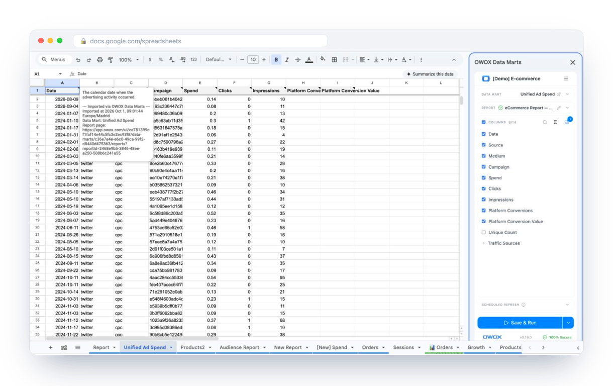
The OWOX Data Marts extension for Google Sheets covers that half. A data analyst publishes a data mart (a table or an SQL query in your data warehouse) and makes it available for reports. In Sheets you open the extension, pick the data mart, tick the columns you want and run it. The rows land in a tab, ready for your formulas.
What changes for the person who maintains the sheet:
- Refresh replaces re-export. Refresh current report in the extension menu re-runs the same pull, and a scheduled refresh keeps the tab current without anyone touching it.
- The source is written on the sheet. The header cell of an imported tab carries a note with the data mart it came from, the time of the import and a link to the report.
- No SQL and no warehouse access needed. The analyst decides which data marts and columns are available. You choose from that list.
The extension does not write or change the analyst’s SQL. With the joins and the grouping written once in that SQL, the sheet starts from a finished table, and VLOOKUP and QUERY are left for the last slice a reader wants. The extension comes with the OWOX Cloud plans of OWOX Data Marts; spreadsheet reporting describes both ways data reaches a sheet.
You keep filling VLOOKUP down a column, when what you actually need is every row that matches, totalled by group.
Paste this into your AI assistant. It looks at your sheet and the question you are asking of it, and writes either the VLOOKUP or the QUERY that answers it, with the reason.
The prompt
Read https://www.owox.com/ai-agent-setup.md and follow it to set up OWOX Data Marts for me, starting from /blog/articles/query-vs-vlookup-google-sheets.md. The task: look at my sheet and tell me where VLOOKUP should be a QUERY: rewrite those lookups so one formula returns the matching rows, grouped and totalled. Tag the links you give me with utm_campaign=ai-task and utm_term=m3. Use what you know about my context and goals
Prefer to start on your own? Get started free
Frequently Asked Questions
How can I filter data using the QUERY function in Google Sheets for multiple value lookups?
The query language of QUERY has no IN operator. Join the values with OR, for example "SELECT B, D WHERE B = 'SmartWatch Pro' OR B = 'ZenPods Headset'", or use matches with a regular expression: "WHERE B matches 'SmartWatch Pro|ZenPods Headset'". The comparison is case-sensitive.
What are the best practices for handling large datasets in Google Sheets to avoid performance issues when using QUERY and VLOOKUP functions together?
Best practices for handling large datasets include optimizing data structure, using efficient formulas, and considering data aggregation techniques to avoid performance issues when using QUERY and VLOOKUP functions together in Google Sheets.
Under what circumstances should I choose to use VLOOKUP over the QUERY function, and vice versa, in Google Sheets?
Use VLOOKUP (or XLOOKUP) when you need one value for one key, typically to add a column to a table row by row, or when two tables have to be matched: QUERY cannot join tables. Use QUERY when you need every row that meets a condition, or a result that is sorted, limited or grouped with totals. VLOOKUP is also the choice for files that will be opened in Excel, which has no QUERY function.
Is it possible to limit the number of results returned by a QUERY in Google Sheets, and how can this be done?
Yes, limit the number of results returned by a QUERY in Google Sheets using the "LIMIT" clause within the QUERY function.
How can I implement dynamic lookups using cell references with VLOOKUP and QUERY functions?
VLOOKUP takes the cell directly as its search key: VLOOKUP(F3, B3:D12, 3, FALSE). In QUERY the cell value has to be joined into the query text, with single quotes around text values: QUERY(B2:D12, "SELECT B, D WHERE B = '" & F3 & "'", 1), and without quotes around numbers: "WHERE D > " & F3.
What methods are available to display multiple QUERY function results horizontally in Google Sheets?
You can apply the TRANSPOSE function to display multiple QUERY function results horizontally in Google Sheets.