ARRAYFORMULA in Google Sheets: how to use array formulas, with examples
ARRAYFORMULA makes one formula return a result for every row of a range. This guide covers the syntax, calculations across columns, IF, VLOOKUP, SUMIF and COUNTIF inside an array formula, open-ended ranges, the functions that do not expand, and the errors you will meet.

ARRAYFORMULA makes a formula that normally works on one cell work on a whole range and return a result for every row. Instead of writing =B3*C3 and copying it down, you write one formula in the first cell:
=ARRAYFORMULA(B3:B11 * C3:C11)
The results fill the cells below. There is nothing to copy, and no row can end up with a different formula from the others.
| You need | Formula |
|---|---|
| Multiply two columns | =ARRAYFORMULA(B3:B11 * C3:C11) |
| Join two columns as text | =ARRAYFORMULA(B3:B12 & " - " & C3:C12) |
| A condition for every row | =ARRAYFORMULA(IF(D3:D11 > 12000, D3:D11 * 0.1, 0)) |
| Look up a whole list of keys | =ARRAYFORMULA(VLOOKUP(F4:F7, B3:D11, 3, FALSE)) |
| A total for each item of a list | =ARRAYFORMULA(SUMIF(C3:C12, F3:F5, D3:D12)) |
| Cover rows that are added later | =ARRAYFORMULA(IF(B3:B = "", , B3:B * C3:C)) |
ARRAYFORMULA syntax
=ARRAYFORMULA(array_formula)
- array_formula: a range, an expression that uses one or more ranges of the same size, or a function that returns more than one cell.
There are two ways to enter it. Type the function name yourself, or write the inner formula and press Ctrl+Shift+Enter (Cmd+Shift+Enter on a Mac): Sheets wraps the formula in ARRAYFORMULA for you.
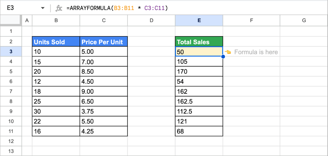
The formula sits in E3 only. E4 to E11 hold results, not formulas: you cannot edit them one by one, and if you type something into one of them, the array formula stops with a #REF! error because it has no room to expand.
Basic operations on columns
Calculate across two columns
Any arithmetic works the same way as with single cells, with ranges in place of the cells:
=ARRAYFORMULA(B3:B11 + C3:C11)
The two ranges have to be the same size. Each row of the result is calculated from the cells of the same row.
Join columns as text
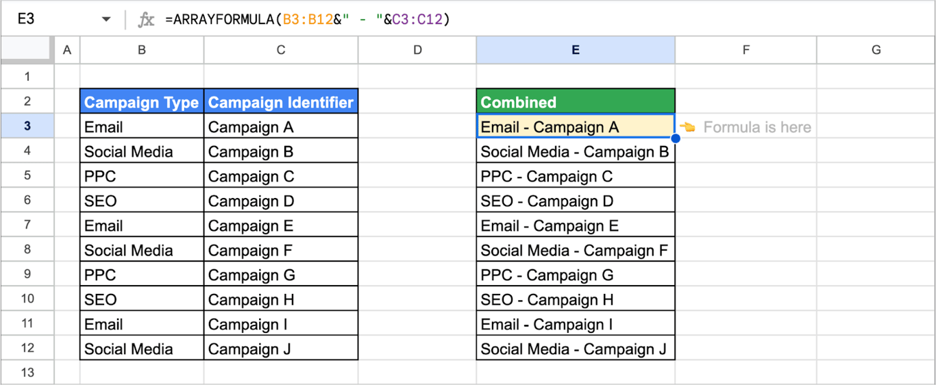
The ampersand joins text, and with ranges it joins row by row. With the campaign type in column B and the campaign name in column C:
=ARRAYFORMULA(B3:B12 & " - " & C3:C12)
Multiply two ranges cell by cell
The ranges can have several columns. Each cell of the first range is combined with the cell in the same position of the second one. With sales for two regions in B3:C5 and the rates for the same regions in D3:E5:
=ARRAYFORMULA(B3:C5 * D3:E5)
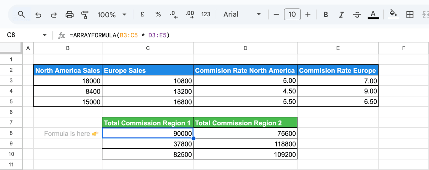
The result is a table of three rows and two columns. This is element-by-element multiplication; for matrix multiplication in the mathematical sense, Sheets has the MMULT function.
OWOX Data Marts
See your first report built in real time. 15 minutes.
- Connect your data warehouse
- Pick your metrics
- Get a live Google Sheets report
In the time it takes to write a ticket. Then imagine never writing that ticket again.
Book a DemoWe'll use your actual use case
ARRAYFORMULA with other functions
ARRAYFORMULA with other functions
IF: a condition for every row
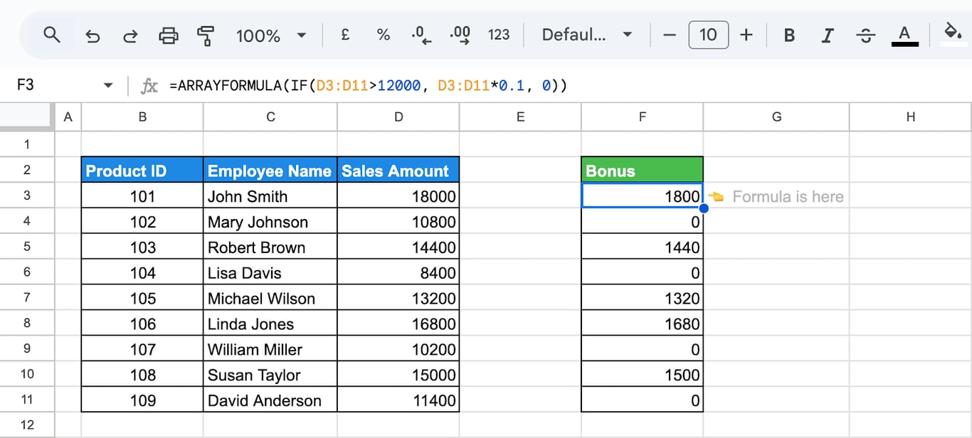
Inside ARRAYFORMULA, IF tests every row of a range and returns a result for each. To pay a 10% bonus on sales above 12,000 and nothing otherwise:
=ARRAYFORMULA(IF(D3:D11 > 12000, D3:D11 * 0.1, 0))
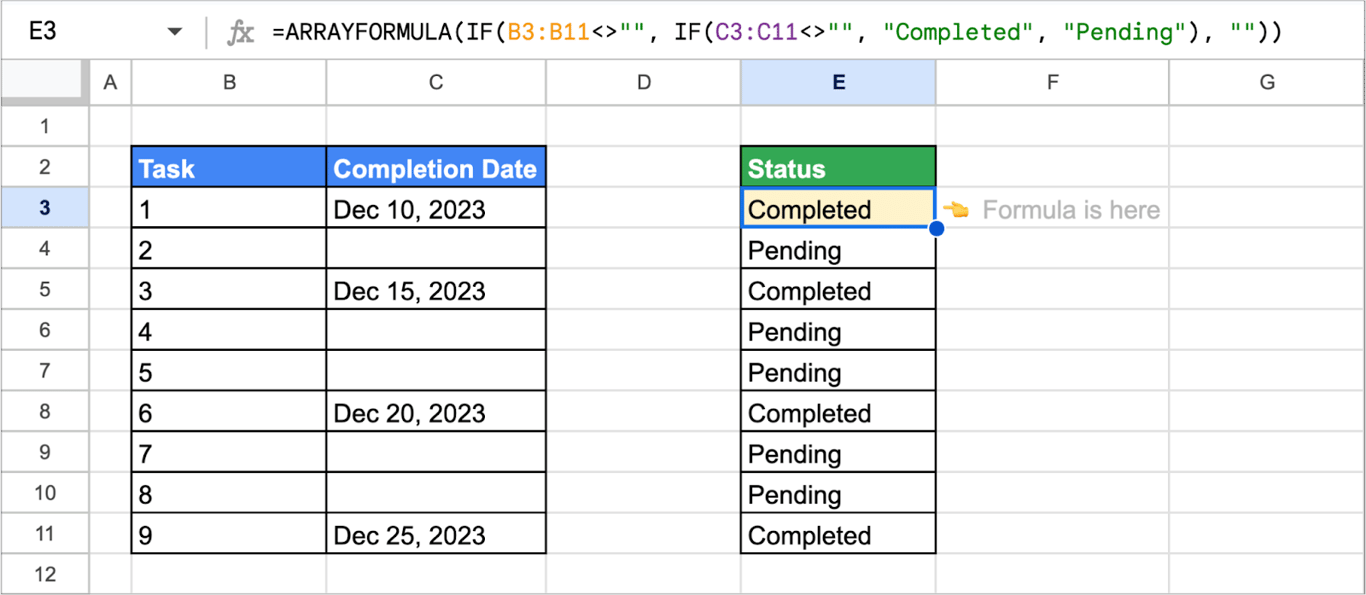
IFs can be nested. This formula leaves the status empty when there is no task, and otherwise shows Completed or Pending depending on whether the completion date is filled in:
=ARRAYFORMULA(IF(B3:B11 <> "", IF(C3:C11 <> "", "Completed", "Pending"), ""))
AND and OR do not work per row. They reduce the whole range to a single TRUE or FALSE, so =ARRAYFORMULA(IF(AND(D3:D5 > 1000, D3:D5 < 2500), "yes", "no")) returns one value for the range. Multiply the conditions for AND and add them for OR:
=ARRAYFORMULA(IF((D3:D5 > 1000) * (D3:D5 < 2500), "yes", "no"))
VLOOKUP: look up a list of keys
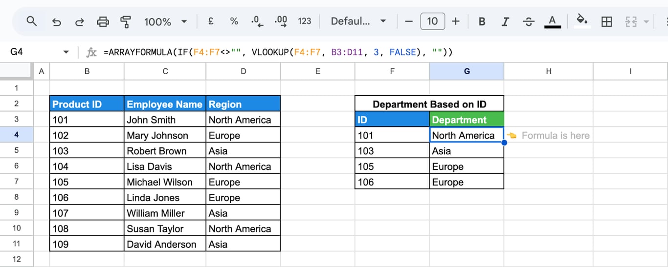
VLOOKUP takes one search key. Inside ARRAYFORMULA it takes a range of keys and returns a result for each. With employee IDs in F4:F7 and the table in B3:D11:
=ARRAYFORMULA(IF(F4:F7 <> "", VLOOKUP(F4:F7, B3:D11, 3, FALSE), ""))
- F4:F7: the IDs to look up.
- B3:D11: the table; the IDs are in its first column.
- 3: the column to return, the region.
- IF(F4:F7 <> “”, …, “”): leaves the result empty where no ID is entered, instead of #N/A.
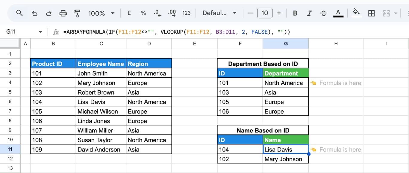
Change the index to 2 and the same formula returns the names:
=ARRAYFORMULA(IF(F11:F12 <> "", VLOOKUP(F11:F12, B3:D11, 2, FALSE), ""))
SUMIF: one total per item
SUMIF returns one total for one criterion. Give it a range of criteria inside ARRAYFORMULA and it returns one total for each of them. With sales reps in C3:C12, amounts in D3:D12 and three names in F3:F5:
=ARRAYFORMULA(SUMIF(C3:C12, F3:F5, D3:D12))
The formula returns three totals, one next to each name.
SUMIF takes one condition. To sum by two columns with it, join the columns and compare them with a joined criterion. This formula adds up revenue for North America in Q1:
=ARRAYFORMULA(SUMIF(D3:D11 & G3:G11, "North America" & "Q1", F3:F11))
- D3:D11 & G3:G11: region and quarter joined row by row, for example North AmericaQ1.
- “North America” & “Q1”: the criterion in the same joined form.
- F3:F11: the revenue to add up.
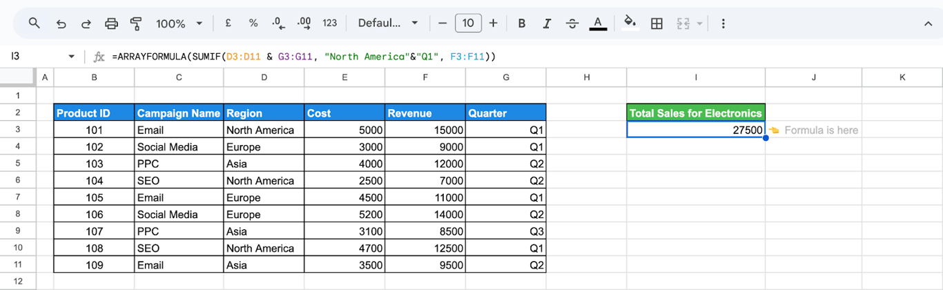
ARRAYFORMULA is required here: without it the joined range is not evaluated row by row. For a single total with several conditions, SUMIFS is the simpler tool and needs no ARRAYFORMULA: =SUMIFS(F3:F11, D3:D11, "North America", G3:G11, "Q1").
SUMIFS does not expand. =ARRAYFORMULA(SUMIFS(D3:D12, C3:C12, F3:F5)) returns a single number, the total for the first criterion, with no error. For a column of totals use SUMIF as above.
COUNTIF: count several values at once
COUNTIF follows the same rule. With a list of criteria in curly braces it returns one count for each:
=ARRAYFORMULA(COUNTIF(B3:C5, {"Product A", "Product B"}))
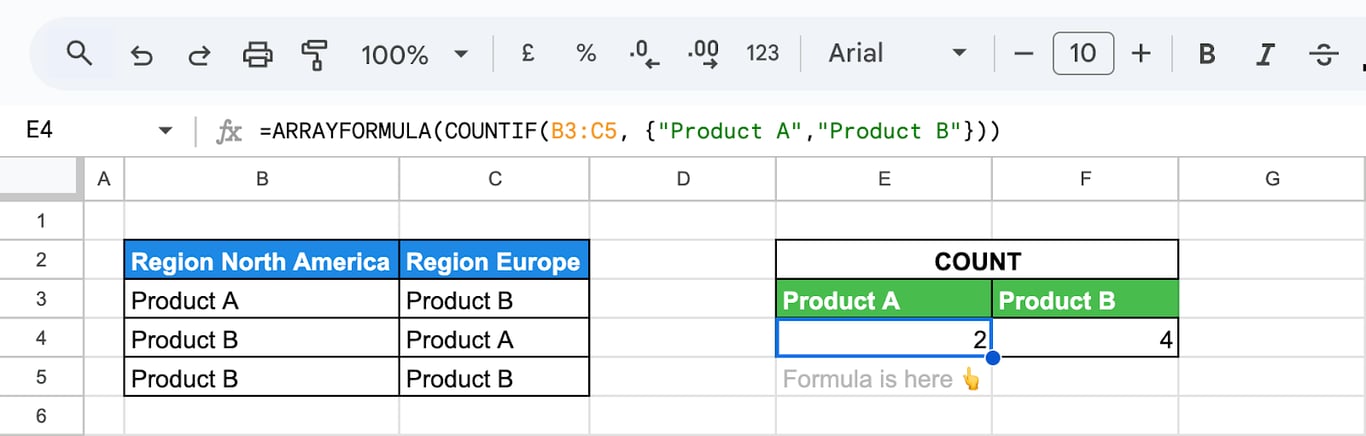
The range B3:C5 contains Product A twice and Product B four times, and the two counts appear side by side, because the criteria are written as a row. Separate them with a semicolon, {“Product A”; “Product B”}, to get the counts one under the other.
FILTER: no ARRAYFORMULA needed
FILTER already returns a range, so it works with or without ARRAYFORMULA around it. To return the rows where the category is Clothing and the region is North America:
=FILTER(C3:F11, (D3:D11 = "Clothing") * (E3:E11 = "North America"))
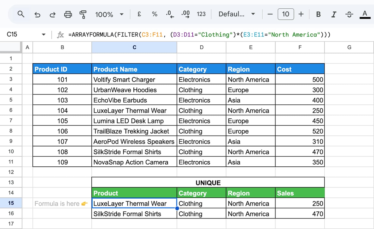
The same goes for removing blanks from a list:
=FILTER(B3:B16, B3:B16 <> "")
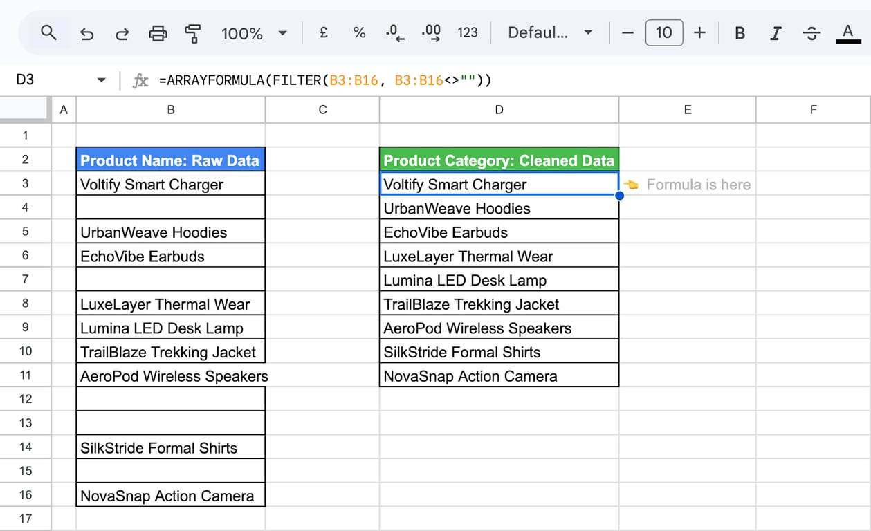
The screenshots show both formulas wrapped in ARRAYFORMULA; the result is the same. QUERY, UNIQUE, SORT and SEQUENCE also return ranges on their own.
CONCATENATE: everything into one cell
CONCATENATE does not work row by row. Inside ARRAYFORMULA it joins the whole range into a single cell:
=ARRAYFORMULA(CONCATENATE(" - " & C3:C11 & ": " & D3:D11 & CHAR(10)))
- ” - “ & C3:C11 & “: “ & D3:D11: product name and description for each row.
- CHAR(10): a line break after each row.
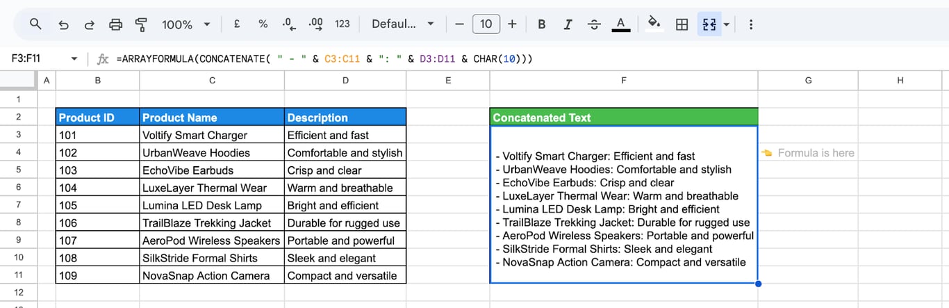
That is useful for a summary cell. For one joined value per row, use the ampersand as in the campaign example above. More on joining text in the guide to CONCATENATE and the ampersand.
Cover rows that are added later
Cover rows that are added later
A range such as B3:B11 stops at row 11. To make the formula pick up new rows, leave the end of the range open and skip the empty rows:
=ARRAYFORMULA(IF(B3:B = "", , B3:B * C3:C))
- B3:B and C3:C: from row 3 to the bottom of the sheet.
- IF(B3:B = “”, , …): returns nothing for rows where column B is empty, so the column is not filled with zeros.
An open-ended formula is calculated for every row of the sheet, including the empty ones. On a sheet with tens of thousands of rows and several such columns, a closed range that is a little longer than the data is faster.
ARRAYFORMULA errors
#REF!: the result has no room
⚠️ Error: #REF! with the message that the array result was not expanded because it would overwrite data.
✅ Solution: One of the cells the formula needs to fill is not empty. Clear the cells below and to the right of the formula.
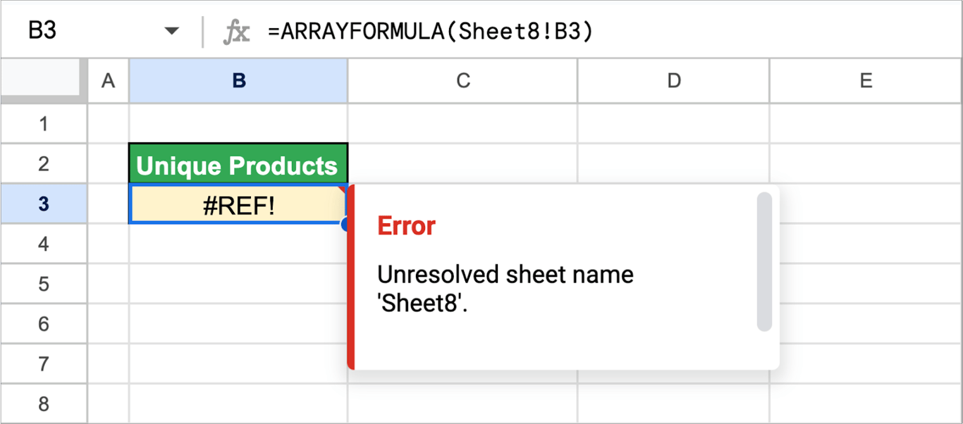
A #REF! with “Unresolved sheet name” is a different problem: the formula points to a tab that does not exist or has been renamed.
An error in one row only
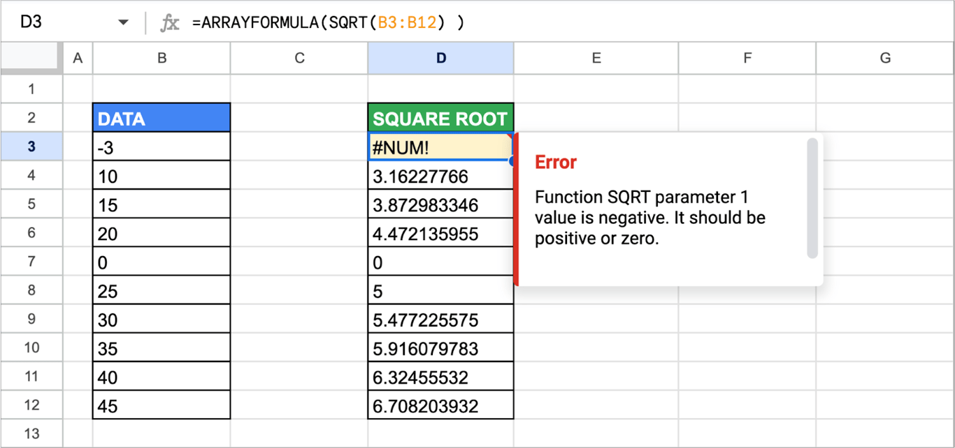
⚠️ Error: One row of the result shows an error such as #NUM! or #DIV/0!, and the others are fine.
✅ Solution: The error belongs to that row’s data. A square root of a negative number returns #NUM!, a division by zero returns #DIV/0!. Fix the value, or wrap the calculation in IFERROR: =ARRAYFORMULA(IFERROR(SQRT(B3:B12), "")).
#N/A: wrong number of arguments
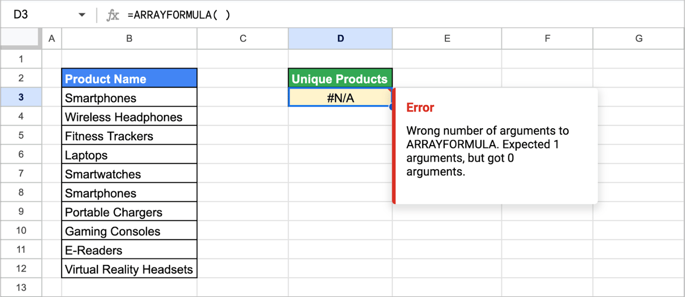
⚠️ Error: #N/A with “Wrong number of arguments to ARRAYFORMULA”.
✅ Solution: The parentheses are empty or contain more than one argument. ARRAYFORMULA takes exactly one.
Inside a lookup, #N/A has its usual meaning: the key was not found.
#ERROR!: the formula cannot be read
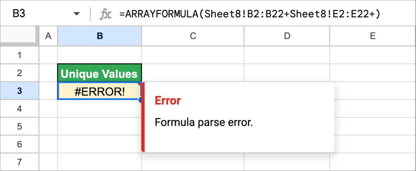
⚠️ Error: #ERROR! with “Formula parse error”.
✅ Solution: Look for a missing parenthesis, a missing quote or an operator with nothing after it.
#VALUE! without ARRAYFORMULA
⚠️ Error: A formula with ranges, such as =SUM(D3:D12 * 2) or =LEN(C3:C5), returns #VALUE!.
✅ Solution: The function expects single values and received ranges. Wrap the formula in ARRAYFORMULA, or press Ctrl+Shift+Enter.
Only one result where a column was expected
⚠️ Error: The formula returns one value and no error.
✅ Solution: The function inside does not expand: AND, OR and SUMIFS reduce the range to one value. Replace AND and OR with multiplication and addition of conditions, and SUMIFS with SUMIF.
Related Google Sheets functions
Related Google Sheets functions
Functions that are often used with or instead of ARRAYFORMULA, each with its own guide:
- FILTER: Returns the rows that meet one or more conditions.
- QUERY: Filters, sorts and summarizes a table with SQL-like syntax.
- UNIQUE: Returns the distinct values of a range.
- XLOOKUP: A lookup that can search in any direction.
- INDEX and MATCH: A lookup built from two functions, for cases VLOOKUP does not cover.
- Pivot tables: Summarize a table by category without formulas.
- QUERY with UNIQUE: Combines SQL-like filtering with deduplication to return only the distinct rows that match a condition.
- QUERY date filtering: Filters rows by a date or a date range inside a QUERY formula.
One formula per column is half the job
One formula per column is half the job
ARRAYFORMULA removes the copied formulas from a report. The other fragile part is the range it runs on. When the rows are pasted in from an export, the formula silently calculates whatever is there: last week’s rows that nobody replaced, a column that shifted by one, numbers that arrived as text.
The OWOX Data Marts extension for Google Sheets covers that half. A data analyst publishes a data mart (a table or an SQL query in your data warehouse) and makes it available for reports. In Sheets you open the extension, pick the data mart, tick the columns you want and run it. The rows land in a tab, ready for your formulas.

What changes for the person who maintains the sheet:
- Refresh replaces re-export. Refresh current report in the extension menu re-runs the same pull, and a scheduled refresh keeps the tab current without anyone touching it.
- The source is written on the sheet. The header cell of an imported tab carries a note with the data mart it came from, the time of the import and a link to the report.
- No SQL and no warehouse access needed. The analyst decides which data marts and columns are available. You choose from that list.
The extension does not write or change the analyst’s SQL. The array formulas then run on rows that come from the same data mart on every refresh. The extension comes with the OWOX Cloud plans of OWOX Data Marts; spreadsheet reporting describes both ways data reaches a sheet.
Turn your data into decisions.
Governed data marts give you the clean foundation ML needs to actually work.
- No AI hallucinations
- Analyst-governed definitions
- Every number traces to SQL
Frequently Asked Questions
How to Use the ARRAYFORMULA Function in Google Sheets?
To use the ARRAYFORMULA function, start with =ARRAYFORMULA(), and inside the parentheses, enter the desired calculation or operation to apply it across a range of cells or data.
Is it Possible to Combine Multiple Array Formulas in Google Sheets, and If So, How?
Yes, you can combine multiple array formulas by nesting them within one another, allowing for more intricate and powerful calculations.
How Do Array Formulas Interact with Other Functions in Google Sheets?
Array formulas can be combined with various functions, such as SUM, AVERAGE, or VLOOKUP, to perform complex calculations and data manipulations.
Are There Any Limitations or Common Errors to Be Aware of When Using Array Formulas in Google Sheets?
Yes. The cells the result needs must be empty, otherwise the formula returns #REF!. AND, OR and SUMIFS do not expand inside ARRAYFORMULA and return a single value; use multiplication of conditions and SUMIF instead. An open-ended range such as B3:B is calculated for every row of the sheet, which slows down large files.
What Is an Array Formula in Google Sheets?
An array formula in Google Sheets is a single formula that can perform calculations or operations on multiple cells or an entire range, simplifying complex data tasks.
How Can I Troubleshoot Issues with My Array Formulas in Google Sheets?
Read the message in the cell. #REF! usually means the result has no room to expand, so clear the cells below the formula. #VALUE! on a formula with ranges means ARRAYFORMULA is missing. #ERROR! is a typing mistake such as a missing parenthesis. An error in a single row comes from that row's data and can be hidden with IFERROR.
How Do I Apply a Formula to a Single Cell in Google Sheets?
Type the formula with cell references, for example =B3*C3, and press Enter. No ARRAYFORMULA is needed. To turn it into an array formula later, replace the cells with ranges and press Ctrl+Shift+Enter.
What Is the Inside Content of an ARRAYFORMULA Function?
The inside content of an ARRAYFORMULA function typically includes the desired calculation or operation, enclosed within the function's parentheses.