
How to Use the REPT Function in Google Sheets for Data Customization
Master the REPT Function in Google Sheets to create custom patterns, enhance data visualization, and improve data presentation effortlessly.


The REPT function in Google Sheets is a versatile tool that simplifies repetitive data tasks by allowing you to repeat a specified text string or character a set number of times.
Whether you're creating visual indicators, customizing cell content, or standardizing data formatting, this function offers a straightforward way to tailor your spreadsheets to your needs.
In this guide, we’ll explore practical applications of the REPT function, from generating bar charts within cells to adding custom text patterns, ensuring your data is both functional and visually impactful. Learn how this simple yet powerful tool can streamline your spreadsheet customization tasks and elevate your data management strategies.
The Key Role of Data Cleanup for Efficient Google Sheets Use
Data cleanup plays a vital role in efficient Google Sheets use by ensuring your data is accurate, consistent, and reliable. Properly cleaned data reduces errors, streamlines analysis, and improves decision-making processes.
Additionally, clean data saves time and appears more professional, which is especially important when presenting it to others. A strong foundation of well-organized data allows functions like REPT to be utilized effectively, helping you customize and manage your spreadsheets with confidence.
Exploring the REPT Function (With Syntax and Examples)
Master text management in Google Sheets with essential functions like REPT. The REPT function repeats text strings a specified number of times, making it a versatile tool for customizing data and creating patterns. In this section, we will explore the syntax and practical examples of the REPT function to enhance your data customization and formatting skills.
REPT Function
The REPT function in Google Sheets repeats a given text string a specified number of times. This is useful for creating patterns, visualizing data, or filling cells with repeated text for formatting purposes.
Syntax of REPT
REPT(text, number_of_repetitions)
Let’s break down what these parameters represent:
- text: The text string to repeat.
- number_of_repetitions: The number of times to repeat the text.
This function is useful for creating repeated patterns or filling cells with repeated text for formatting and visualization.
Example of REPT
Let’s say you have Product Name details in column C and want to repeat each product name three times in column E for visualization or formatting purposes.
Syntax:
=REPT(C3, 3)

Here:
- C3: Refers to the cell containing the product name.
- 3: Specifies the number of times the product name should be repeated.
This formula generates repeated strings of the product names in column E, creating a consistent and patterned output.
Simple Examples of Using the REPT Function in Google Sheets
The REPT function in Google Sheets simplifies data handling by allowing you to repeat text strings a specified number of times, making it useful for creating patterns, placeholders, or visual aids. In this section, we’ll explore practical examples that demonstrate how the REPT function works and how it can enhance your spreadsheet workflows.
Repeating Text Based on Cell References using REPT
The REPT function dynamically repeats text based on values in other cells, making it ideal for creating customized patterns or data outputs. It simplifies tasks like repeating identifiers, product names, or labels according to specific quantities, ensuring dynamic and flexible formatting for reports, analysis, or data visualization.
Example:
Let’s say you have Order ID data in column B and quantities in column C. You want to repeat each Order ID based on the corresponding quantity in column C.
Use the following formula in a new cell:
=REPT(B3, C3)

Here:
- B3: Refers to the cell containing the text to repeat (Order ID).
- C3: Specifies the number of repetitions for the text in B3.
This formula generates repeated Order IDs in column E, producing results like "10011001" for a quantity of 2, making the data dynamic and easier to analyze.
Adding Decorative Elements for Visual Breaks with REPT
The REPT function in Google Sheets allows you to add decorative elements for visual breaks within your data. By repeating characters such as dashes or stars, you can create separators or section dividers, improving the readability and organization of your spreadsheet without relying on additional formatting tools.
Example:
Let’s say you want to insert a repeated pattern of decorative symbols in column G to create a visual break for better report readability.
Use the following formula in a cell:
=REPT("✂ ", 20)

Here:
- "✂ ": Refers to the character or symbol to be repeated.
- 20: Specifies the number of repetitions for the symbol.
This formula produces repeated symbols in column G, enhancing the visual appeal and organization of the dataset for presentations or printed reports.
Advanced Examples of Using the REPT Function in Google Sheets
Expanding on the basics, these advanced examples demonstrate how the REPT function can be combined with other formulas to tackle more complex tasks. From generating visual patterns and placeholders to creating dynamic text-based indicators, these examples showcase the versatility of the REPT function in solving intricate spreadsheet challenges effectively.
Applying Logical Conditions with REPT
The REPT function in Google Sheets can also be used with logical conditions to create dynamic outputs. It helps display specific text based on a condition, simplifying spreadsheet data evaluation.
Example:
Let’s say you have item prices in Column C and you want to display "Yes" in Column E for prices greater than 200.
Use the following formula in a new cell:
=REPT("Yes", C3 > 200)
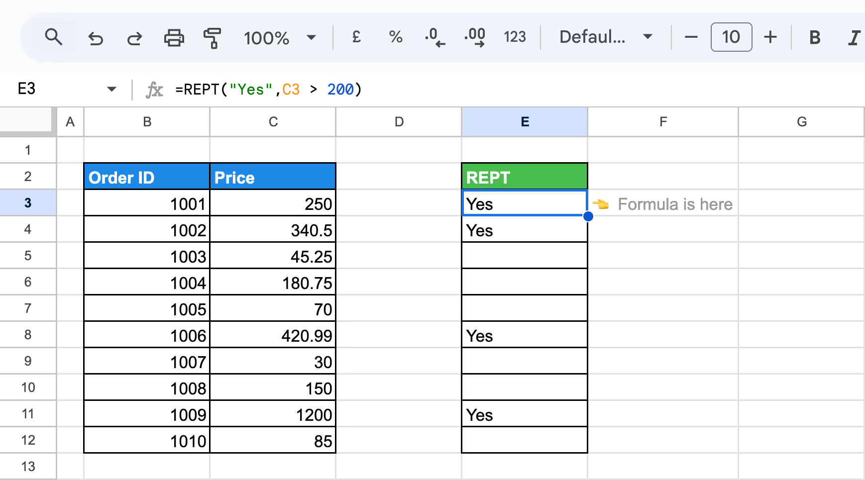
Here:
- C3: Refers to the cell containing the price.
- C3 > 200: Logical condition that checks if the value in C3 is greater than 200.
- REPT("Yes", ...): Returns "Yes" if the condition is true; otherwise, it returns a blank cell.
This formula evaluates each price in Column C and displays "Yes" in Column E for values exceeding 200, leaving other cells blank.
Combining the REPT Function with Other Functions
Combining the REPT function with other Google Sheets functions can greatly enhance your data customization and analysis. This integration allows for more advanced operations, such as creating dynamic text patterns, visual indicators, or placeholders, helping streamline workflows and maintain accurate, well-organized datasets across your spreadsheets.
Using IF for Applying Conditional Formatting with TEXT and REPT
Using the IF function with TEXT and REPT allows you to apply conditional formatting based on specific text values or criteria. This combination enables you to create dynamic outputs, such as visual indicators (e.g., progress bars) or customized messages, depending on the condition being met.
Example of IF with TEXT:
Let’s say you have Total Purchases ($) in column D, and you want to categorize purchases over $3,000 as "High" and those below $3,000 as "Low". You can create a helper column with the following TEXT formula:
=IF(D3>3000, TEXT(D3, "#,##0") & " High", TEXT(D3, "#,##0") & " Low")
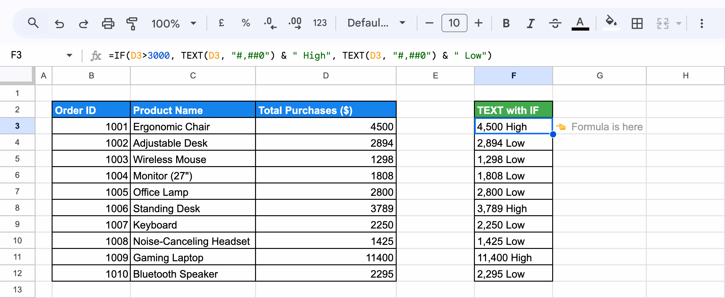
Here:
- IF(D3>3000, ... , ...): The IF function checks if the value in D3(Total Purchases) is greater than $3,000. If true, it executes the first part of the formula; if false, it executes the second part.
- TEXT(D3, "#,##0"): This part formats the value in (Total Purchases) as a number with thousands separators.
- & " High": If the value is greater than $3,000, this part appends the label "High" to the formatted number.
- & " Low": If the value in D3 is less than or equal to $3,000, this part appends the label "Low" to the formatted number.
This formula effectively categorizes sales data as "High" or "Low" based on a specified threshold, formatting the values with thousands of separators for readability.
Example of IF with REPT:
Let’s assume you want to create a visual rating system for each product based on its Total Purchases ($). We’ll rate products with purchases over $3,000 with 5 full stars (★), and products with purchases below or equal to $3,000 will get 5 empty stars (☆).
Use the following formula to rate the performance:
=IF(D16>3000, REPT("★", 5), REPT("☆", 5))
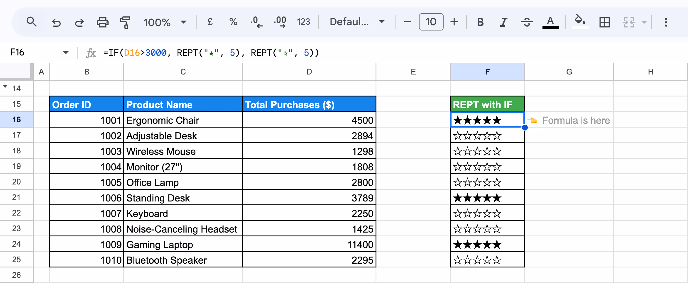
Here:
- IF(D16>3000, ... , ...): Checks if the sales value in D(Total Purchases) is greater than $3,000. If true, it will display 5 full stars (★). If false, it will display 5 empty stars (☆).
- REPT("★", 5): Repeats the full star symbol 5 times to represent high sales performance visually.
- REPT("☆", 5): Repeats the empty star symbol 5 times for products with lower sales.
By using the REPT function with IF statements, you can visually represent data performance, such as figures, with symbols like stars.
💡 Want to master the IF function in Google Sheets? Check out our detailed article to learn how to apply conditional logic to your data, automate tasks, and make smarter decisions. Don't miss out on valuable insights! Read the full article here.
Combining LEN and REPT for Padding Text Strings
LEN and REPT functions in Google Sheets allows you to pad text strings with additional characters to achieve a desired length. LEN helps measure the current length of a string, while REPT repeats a specified character to fill the gap.
Example:
Suppose you have product names that you want to pad with underscores to make all the product names uniform in length. By using the LEN and REPT functions, you can ensure the text strings are all 24 characters long.
Use this formula:
=C3 & REPT("_", 24 - LEN(C3))
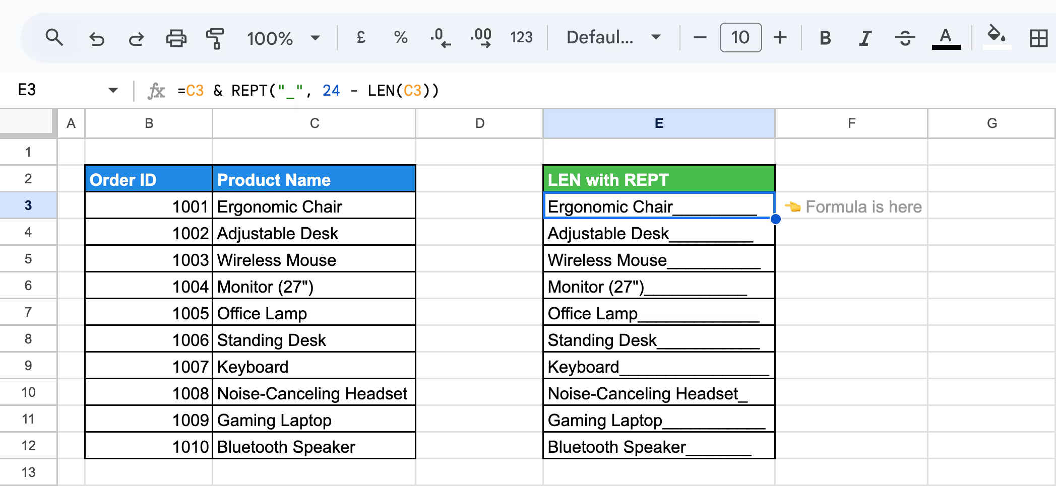
Here:
- LEN(C3): This calculates the length of the text in C3(the product name).
- REPT("_", 24 - LEN(C3)): Adds enough underscores to the end of the product name to make the total length equal to 24 characters.
- C3 & REPT(...): Combines the original product name with the appropriate number of underscores.
By using the LEN and REPT functions, you can pad product names (or any text) to a specific length, ensuring uniformity in the data.
Repeating Images Dynamically with REPT with SPLIT
Repeating images dynamically in Google Sheets can be useful for visualizing data such as product catalogs, customer profiles, or report templates. By combining the REPT, SPLIT, and IMAGE functions, you can automate the process of repeating an image a specified number of times across multiple rows.
Example:
Suppose, if you're creating a dataset where each product requires its image to be displayed repeatedly across several rows, you can automate this process using the REPT, SPLIT, and IMAGE functions together.
Use this formula:
=ARRAYFORMULA(IMAGE(SPLIT(REPT("https://tse3.mm.bing.net/th?id=OIP.iLaBmVMgnUJD2uZkTD64cQHaHa&pid=Api&P=0&h=180"&"♕", 3), "♕")))
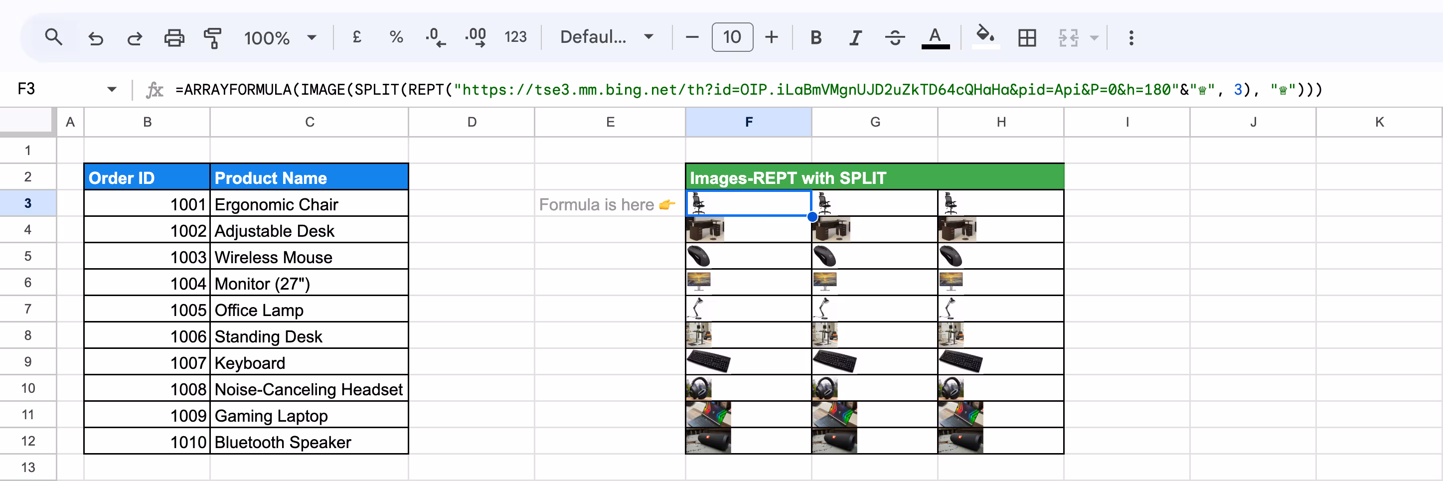
Here:
- REPT("https://tse3.mm.bing.net/th?id=OIP.iLaBmVMgnUJD2uZkTD64cQHaHa&pid=Api&P=0&h=180"&"♕", 3): Repeats the image URL -3 times, separating each repetition with the delimiter "♕".
- SPLIT(..., "♕"): The SPLIT function separates the repeated image URLs at each "♕" delimiter into individual cells.
- IMAGE(...): The IMAGE function renders the image from each URL into the corresponding cells.
- ARRAYFORMULA: Applies the formula across multiple rows, ensuring each repeated image is displayed vertically in separate cells.
This approach allows you to efficiently repeat and display the same image across multiple rows, saving time and maintaining consistency.
Using REPT with SPLIT and TRANSPOSE for Repeated Text
Using the REPT, SPLIT, and TRANSPOSE functions together in Google Sheets allows you to repeat a text value multiple times and display it across multiple rows. This method helps efficiently create vertical lists from repeated data, making it ideal for tasks like data replication or tracking customer interactions.
Example:
Suppose you have a customer name in cell C3 and the number of repetitions you want in cell D3. You can use the formula to repeat the customer name multiple times and split it into separate rows. This can be useful for cases where you need to replicate data across rows for analysis.
Use this formula:
=TRANSPOSE(SPLIT(REPT(C3&"♕", D3), "♕"))
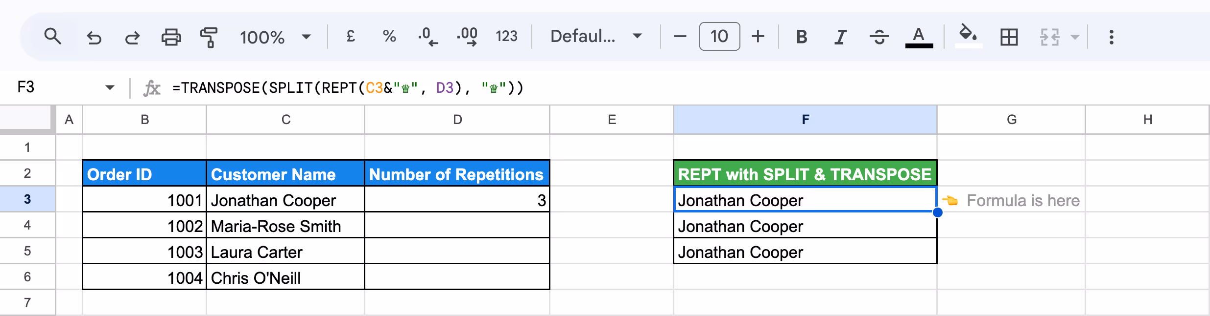
Here:
- REPT(C3&"♕", D3): Repeats the value in C3 ("Jonathan Cooper") D3 times, with a delimiter "♕" in between. If D3 = 3, the result will be: "Jonathan Cooper♕Jonathan Cooper♕Jonathan Cooper".
- SPLIT(..., "♕"): The SPLIT function splits the repeated string at each "♕" delimiter into separate cells. It will result in an array like this:
- TRANSPOSE: The TRANSPOSE function converts the horizontal array into a vertical list, which will output one name per row.
By using this method, you can automate the repetition of customer names (or any text) for reporting, tracking, and analysis purposes.
Creating Bar Charts Using REPT and CHAR Functions
This technique allows you to create visual bar charts within cells using the REPT and CHAR functions. By repeating a specific character or emoji, you can represent quantities or values, creating a simple yet effective way to visualize data in a spreadsheet.
Example:
Suppose you have product quantities, and you want to represent these quantities using text-based bar charts visually. You can use the REPT and CHAR functions to repeat a specific character for each value in the Quantity column.
Use this formula:
=REPT(CHAR(10074), D3)
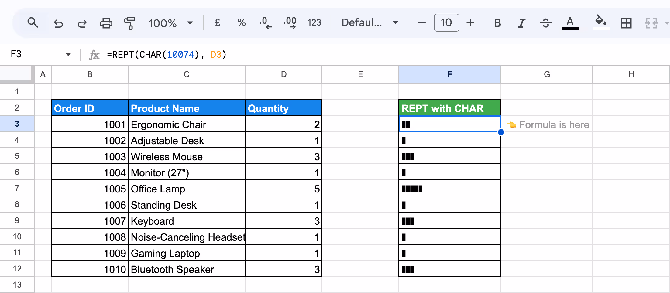
Here:
- CHAR(10074): This function returns the heavy vertical bar emoji (❚), which is used as the "block" in the bar chart.
- REPT(CHAR(10074), D3): The REPT function repeats the ❚ character as many times as the quantity in cell D3 (which corresponds to the Quantity column).
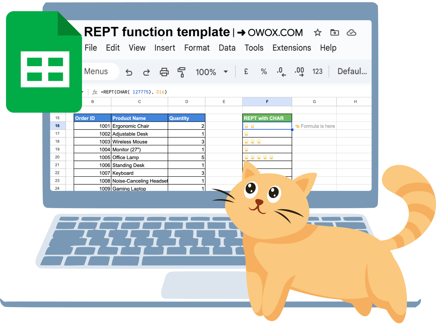
In another variation, we’ll use the Star emoji (⭐) to represent quantities to know which products are sold the most, for being a star product. By applying the REPT and CHAR functions with the Star emoji's Unicode, we can visually display the data more dynamically.
Use this formula:
=REPT(CHAR( 127775), D15)

Here:
- CHAR(127775): This returns the Star emoji (⭐), which will be used as the "block" in the bar chart.
- REPT(CHAR(127775), D15): The REPT function repeats the Star emoji (⭐) based on the Quantity in cell D15 (corresponding to the Quantity column in your dataset).
Let's look at another possible example: suppose you want to create a vertical bar chart using the Circle emoji (●) in Google Sheets, with each cell in a range displaying a series of circles representing the quantity value.
Use this formula:
=ArrayFormula(JOIN(CHAR(10), REPT(CHAR(9679), D27:D36)))
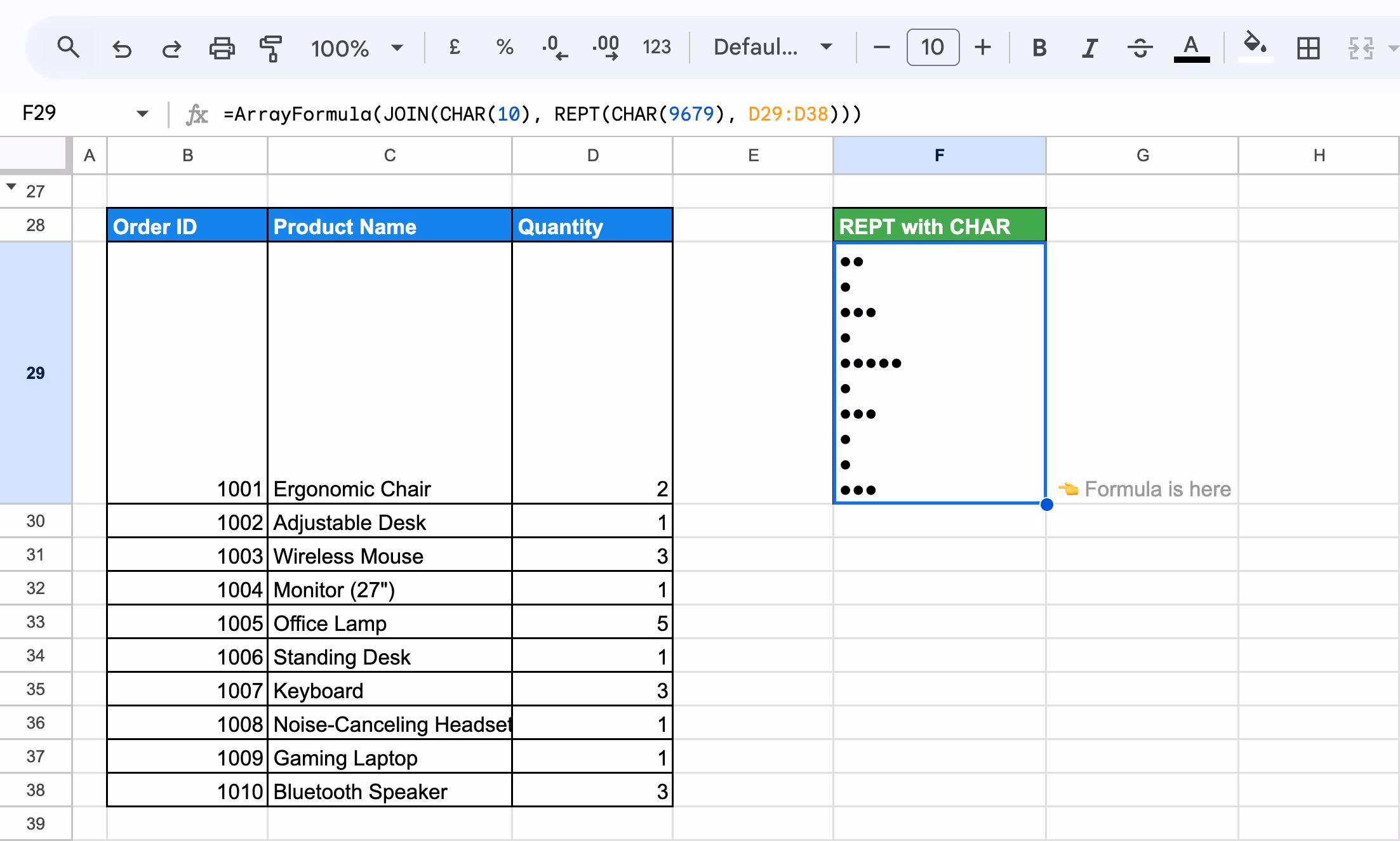
Here:
- CHAR(9679): This returns the Circle emoji (●), which acts as the "block" in the bar chart.
- REPT(CHAR(9679), D27:D36): The REPT function repeats the Circle emoji (●) based on the quantity in each cell from D27 to D36.
- JOIN(CHAR(10), ...): The JOIN function combines the repeated emojis with line breaks (CHAR(10)), stacking the circles vertically for each value in the range.
By combining ArrayFormula, JOIN, and REPT with CHAR, you can create dynamic, text-based vertical bar charts in Google Sheets.
Visualizing Participation Status with REPT and COUNTIF
This method allows you to easily visualize participation or completion status by using symbols, like asterisks (*), to represent completed actions. By combining REPT with COUNTIF, you can dynamically generate visual cues based on the number of completed tasks or conditions met within your dataset.
Example:
For example, a customer activity or order status dataset where each column represents a task or action, and the presence of "Y" in a cell indicates that the action was completed. You can use the REPT with COUNTIF to visually represent each order's completion status.
=REPT("*", COUNTIF(D3:H3, "Y"))
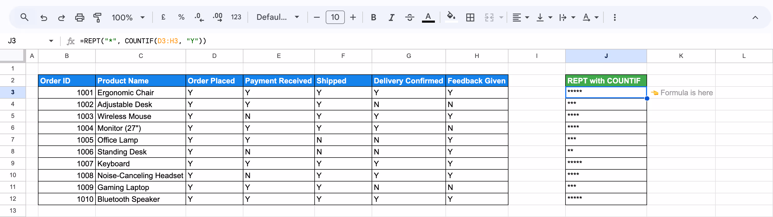
Here:
- D3:H3: Represents the range of cells for each order, where each column indicates a task (e.g., Order Placed, Payment Received, Shipment Processed, Delivery Confirmed, Feedback Given).
- COUNTIF(D3:H3, "Y"): Counts how many times "Y" appears in the row (i.e., how many tasks are completed).
- REPT("*", COUNTIF(D3:H3, "Y")): Repeats the asterisk (*) the number of times equal to the number of completed tasks (the "Y" values).
By using REPT and COUNTIF, you can easily visualize the progress or completion of multiple tasks or actions for each order or customer.
💡 Want to learn more about using COUNTIF and COUNTIFS in Google Sheets? Check out this comprehensive guide on COUNTIF and COUNTIFS Functions in Google Sheets to enhance your data analysis skills and effectively filter and count data based on specific conditions.
Troubleshooting Common Issues with REPT Function
When using the REPT function, you may encounter errors like #VALUE!, #N/A, or #NAME. These issues often arise due to incorrect data types or errors in function syntax. In this section, we’ll examine these common errors and provide solutions to help you resolve them effectively.
#VALUE! Error
⚠️ Error: The #VALUE! error in the REPT function occurs when the resulting text exceeds 32,767 characters. This happens if the number of repetitions or the length of the text string is too large.
✅ Solution: To fix this issue, reduce the number of repetitions or shorten the text string to ensure the total output stays within the 32,767-character limit. This will prevent the error and ensure the function works as expected.
Using a Negative Number of Repetitions in REPT
⚠️ Error: The number_of_repetitions argument in the REPT function must be a non-negative integer. If a negative number is provided, REPT will return an error.
✅ Solution: Ensure that the number_of_repetitions argument is a positive integer or zero. If you are dynamically calculating the repetitions, add a check to ensure the value is non-negative before passing it to the REPT function.
Providing a Non-Numeric Value for Number of Repetitions
⚠️ Error: The number_of_repetitions argument in the REPT function must be a non-negative integer. If a non-numeric value (such as text or a blank cell) is provided, REPT will return an error.
✅ Solution: Ensure that the number_of_repetitions argument is a valid numeric value. If you're using a reference to a cell, verify that the cell contains a numeric value and not text or an empty cell. You can also use error handling (e.g., IF or ISNUMBER) to check for valid inputs before using REPT.
Best Practices for Using REPT Function
When using the REPT function in Google Sheets, applying it effectively is essential for maintaining organized and accurate data. This section outlines best practices for leveraging the REPT function to create patterns, placeholders, or visual aids, helping you streamline your data management and customization processes.
Combining with Other Functions for Advanced Text Patterns
Enhance text manipulation by combining the REPT function with other Google Sheets functions. For example, use REPT to repeat text strings based on specific conditions or to create visual patterns like progress bars. Integrating REPT with other functions enables more advanced and dynamic data customization, streamlining complex spreadsheet tasks.
Use Conditional Formatting
Use the REPT function to visually enhance progress bars or create patterns in your data. By combining REPT with conditional formatting, you can make progress indicators or repeated text elements more visually intuitive, ensuring your data remains well-organized and easy to interpret.
Generate Large Test Data Sets with REPT
Use the REPT function to quickly generate large test datasets by repeating text or values a specified number of times. This is helpful for simulating data in scenarios like testing formulas, creating placeholders, or conducting stress tests on your Google Sheets model.
Essential Google Sheets Functions for Advanced Data Analysis
Google Sheets offers a wide variety of powerful functions that simplify data analysis, enabling users to easily handle and interpret large datasets. These essential functions help you extract insights, manage data efficiently, and perform in-depth analysis with minimal effort.
- UNIQUE: Extracts unique values from a range, removing duplicates to give you a cleaner dataset.
- IMPORTRANGE: Imports a specific range of cells from another spreadsheet, making consolidating data across multiple sheets easy.
- MATCH: Searches for a value within a range and returns the relative position of that value, aiding in lookups and data comparison.
- COUNTA: Counts the number of non-empty cells in a range, useful for tracking data presence or tallying entries.
- MAX, MIN, MEDIAN: These functions allow you to find the highest value (MAX), the lowest value (MIN), or the middle value (MEDIAN) in a dataset, essential for summary statistics.
- TIME: Converts hours, minutes, and seconds into a time value, simplifying time-based calculations.
- WORKDAY: Calculates a date that is a specified number of working days (excluding weekends and holidays) from a given date.
- ROUND: Rounds a number to a specified number of digits, useful for formatting and presenting data consistently.
Visualize Your Data with OWOX: Reports, Charts, and Pivot Tables
The REPT function is great for repeating text or numbers, but what if you could automate even more? The OWOX Reports lets you create dynamic reports, charts, and data visualizations effortlessly, saving you time and boosting productivity.
Take your data customization to the next level with tools that simplify workflows and deliver results faster. Install the OWOX Reports Extension today and experience the power of automated data handling!
Frequently asked questions


Finally, a tool that doesn't ask business users to learn a new dashboarding UI. Our marketing team already knows Sheets. OWOX just delivers the right data.
Joinable data marts concept was the thing that sold us. We can now use the semantic layer without building one.
Self-hosted the OSS version on Digital Ocean. Zero vendor lock-in. Contributed a Shopify connector back in week two.