UNIQUE function in Google Sheets: syntax, examples and common errors
UNIQUE returns the distinct rows of a range and leaves the source data untouched. This guide covers the syntax, the difference between distinct and exactly-once values, drop-down lists without duplicates, combinations with SORT, FILTER, SUMIF, COUNTA and QUERY, and the errors UNIQUE returns.

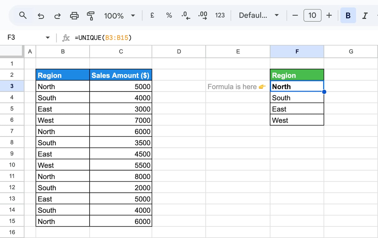
The UNIQUE function in Google Sheets returns the distinct rows of a range, in the order they first appear. Type =UNIQUE(B3:B15) next to your data and you get every value from B3:B15 once, with the duplicates left out. The source data stays untouched.
This guide covers the syntax, the difference between distinct and exactly-once values, worked examples (several columns, horizontal data, drop-down lists), combinations with SORT, FILTER, SUMIF, COUNTA and QUERY, and the errors UNIQUE returns.
Note: Originally published in February 2024. Fully updated in October 2026: repeated sections merged, the error examples corrected, and advice that applied to Excel rather than Google Sheets removed.
UNIQUE function syntax
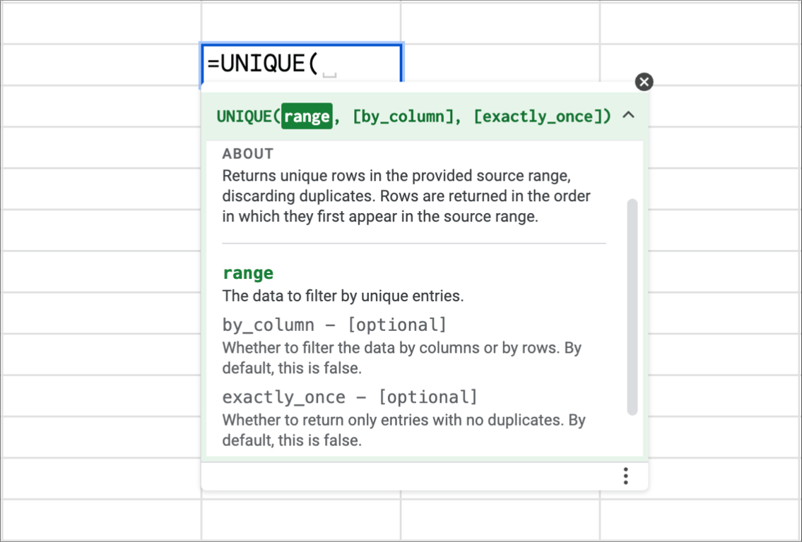
=UNIQUE(range, [by_column], [exactly_once])
- range: the data to filter.
- by_column (optional): whether to compare columns instead of rows. FALSE by default, which compares rows.
- exactly_once (optional): whether to return only the entries that appear exactly once. FALSE by default, which returns every distinct entry.
Three things to know before the examples:
- UNIQUE compares whole rows. With a range of two columns, a row is a duplicate only if both cells match.
- It keeps the original order. Wrap it in SORT if you need another one.
- The result spills into the cells below and to the right of the formula, so they must be empty.
Distinct values and unique values are not the same
Distinct values and unique values are not the same
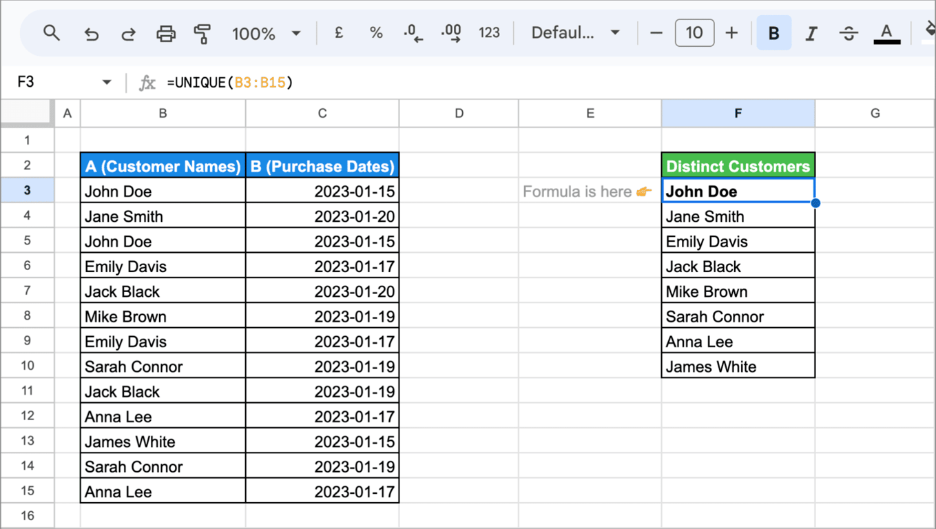
By default UNIQUE returns distinct values: every value once, however many times it appears. With exactly_once set to TRUE it returns unique values in the strict sense: only the values that appear a single time.
Take a list of customers with one row per purchase. This lists every customer once:
=UNIQUE(B3:B15)
And this lists only the customers who bought exactly once:
=UNIQUE(B3:B15,,TRUE)
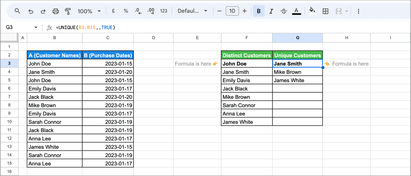
The two commas skip the by_column argument. The first result answers “who are our customers”, the second “who never came back”.
OWOX Data Marts
See your first report built in real time. 15 minutes.
- Connect your data warehouse
- Pick your metrics
- Get a live Google Sheets report
In the time it takes to write a ticket. Then imagine never writing that ticket again.
Book a DemoWe'll use your actual use case
UNIQUE function examples
List the distinct values of a column
A table of advertising campaigns has the ad type in column E. To see which ad types are in use:
=UNIQUE(E3:E15)
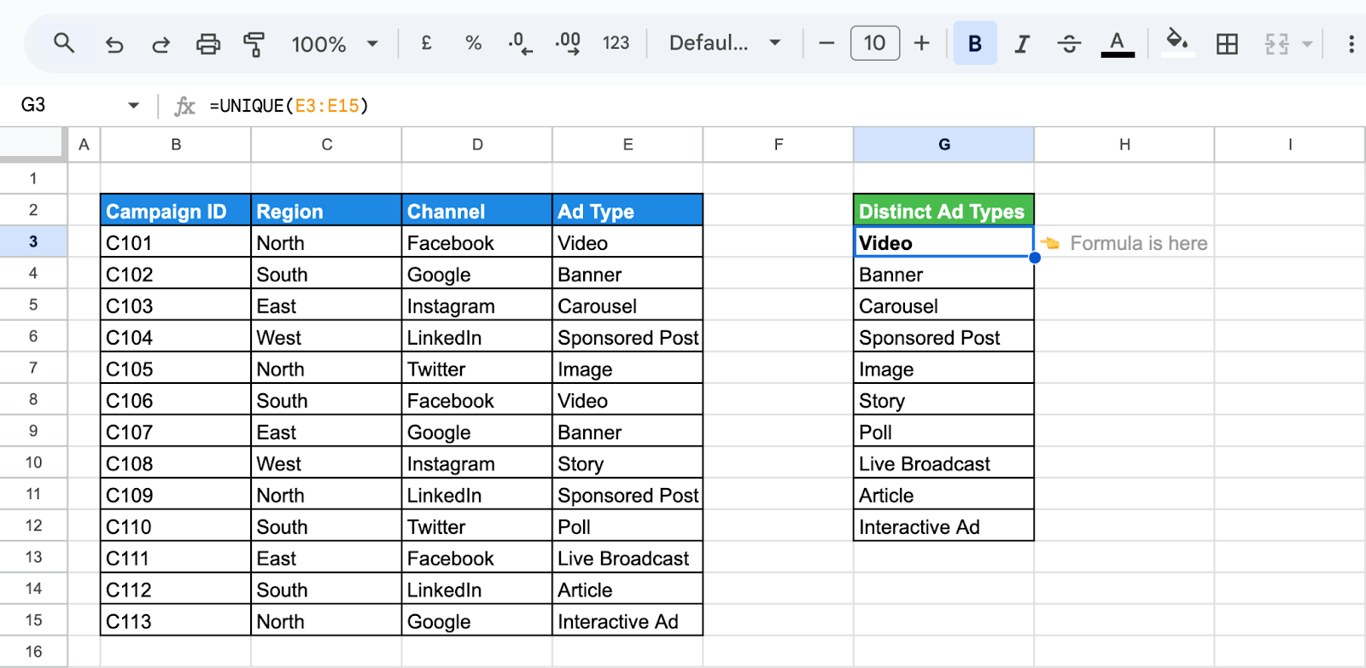
To cover a whole column, including rows added later, use an open range such as =UNIQUE(E3:E).
💡 UNIQUE returns a clean copy and leaves the source as it is. To delete the duplicate rows themselves, see our guide on how to remove duplicates in Google Sheets.
Distinct rows across several columns
With customer names in column B and purchase dates in column C, this returns each customer and date pair once:
=UNIQUE(B3:C15)
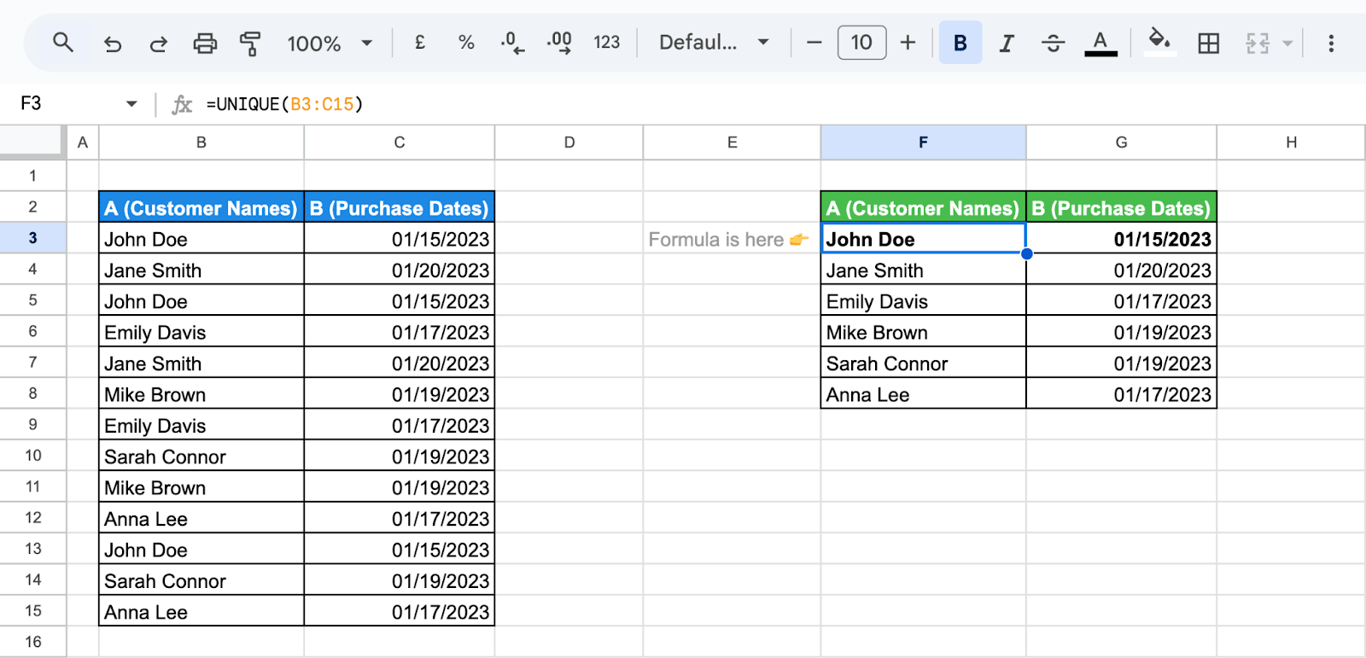
A customer who bought on two different days appears twice, because the rows differ in the date.
Distinct columns in horizontal data
When each campaign is a column instead of a row, set by_column to TRUE and UNIQUE compares the columns:
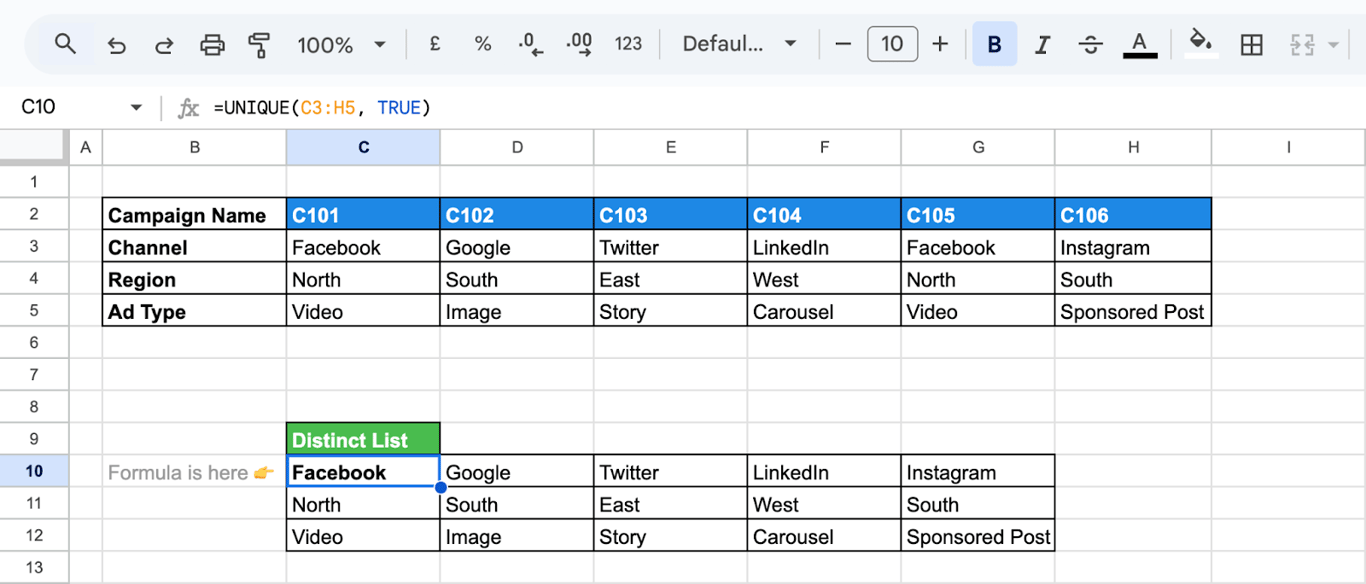
=UNIQUE(C3:H5, TRUE)
Campaigns with the same channel, region and ad type collapse into one column, which shows at a glance which setups are repeated.
A drop-down list without duplicates
A drop-down built from a raw column repeats every value. Build it from a UNIQUE list instead.
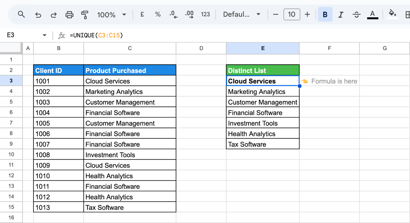
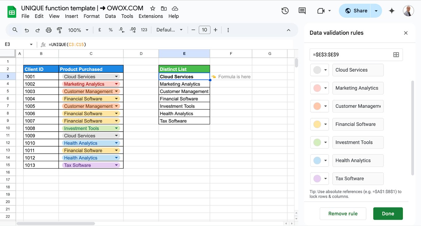
1. In an empty column, list the distinct products with =UNIQUE(C3:C15). Here the formula is in cell E3.
2. Select the cells that should get the drop-down.
3. Go to Data → Data validation and add a rule.
4. Under Criteria, choose Dropdown (from a range) and enter the range of the distinct list, here E3:E9.
5. Click Done.
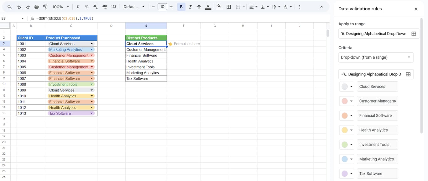
For an alphabetical drop-down, sort the list first with SORT:
=SORT(UNIQUE(C3:C15), 1, TRUE)
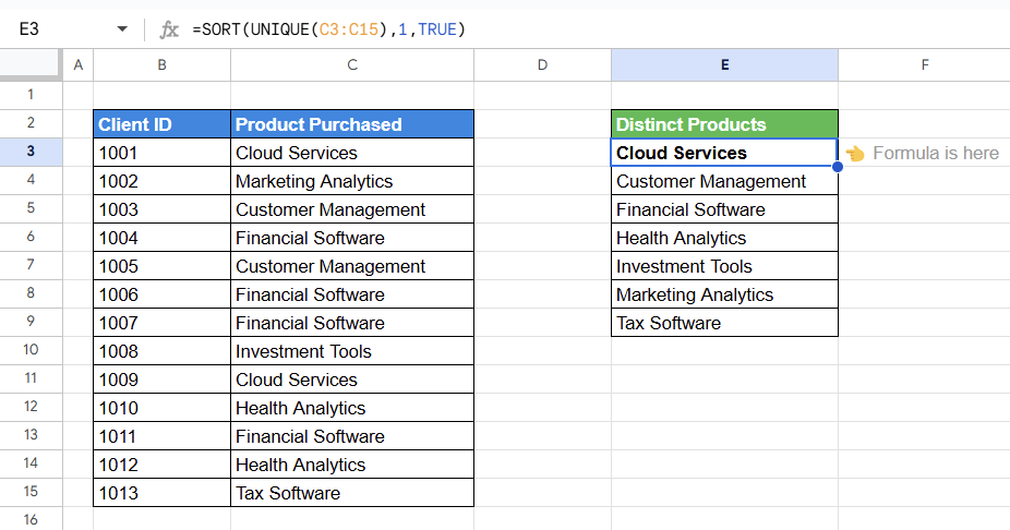
The 1 is the column to sort by and TRUE means ascending order. The drop-down then follows the sorted list.
💡 To summarize the same data by category instead of listing it, see our guide to pivot tables in Google Sheets.

Combining UNIQUE with other functions
Combining UNIQUE with other functions
UNIQUE and TEXTJOIN: the distinct values in one cell
TEXTJOIN joins an array into one string. Feed it the output of UNIQUE to list, for example, every channel used in your campaigns in a single cell:
=TEXTJOIN(", ", TRUE, UNIQUE(B3:B15))
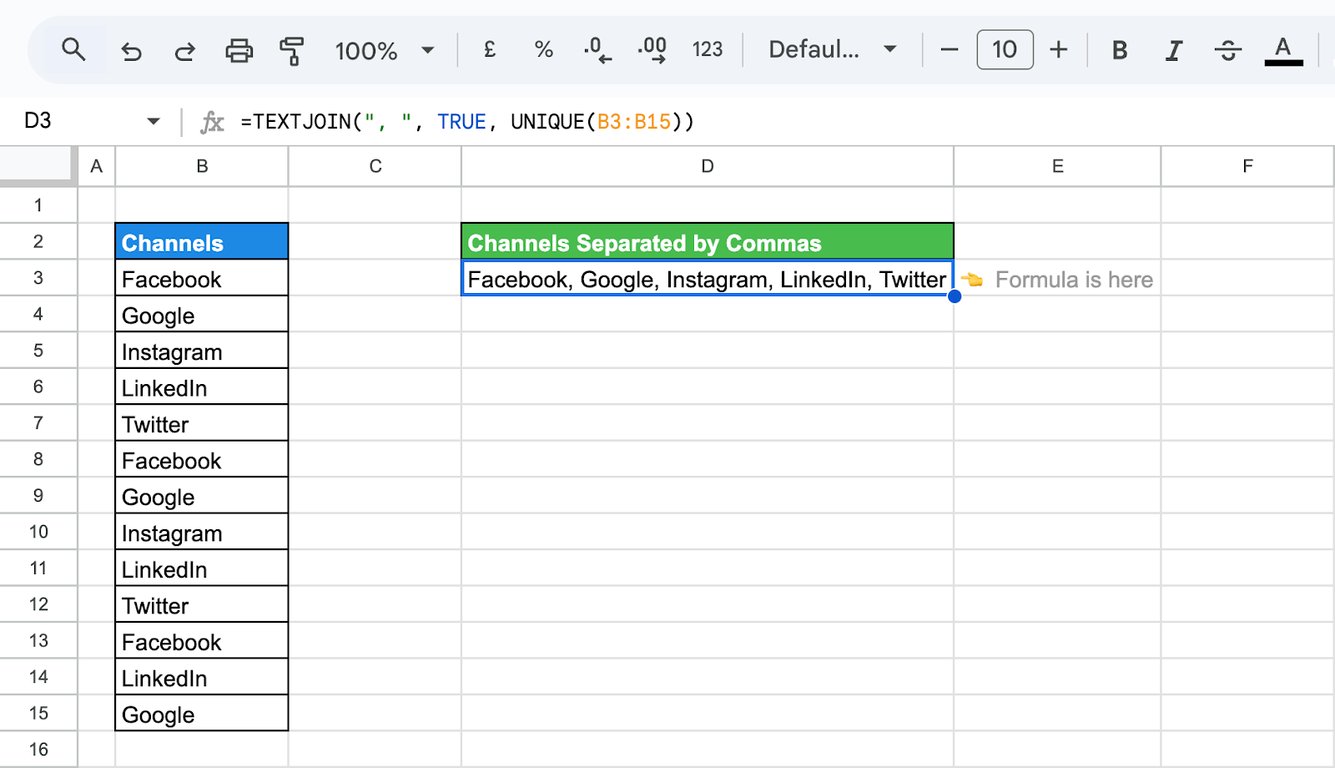
- UNIQUE(B3:B15): returns the distinct values of the range.
- TEXTJOIN(“, “, TRUE, …): joins them with a comma and a space. TRUE skips empty cells.
UNIQUE and SUMIF: a total per distinct value
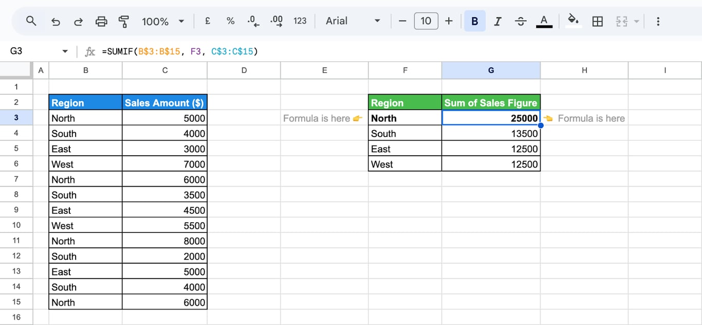
To sum sales per region:
1. List the regions once with =UNIQUE(B3:B15), here in cell F3.
2. Next to the first region, add up its sales:
=SUMIF(B$3:B$15, F3, C$3:C$15)
3. Drag the formula down to the last region. The dollar signs keep the ranges fixed while F3 moves.
UNIQUE and COUNTA: how many distinct values
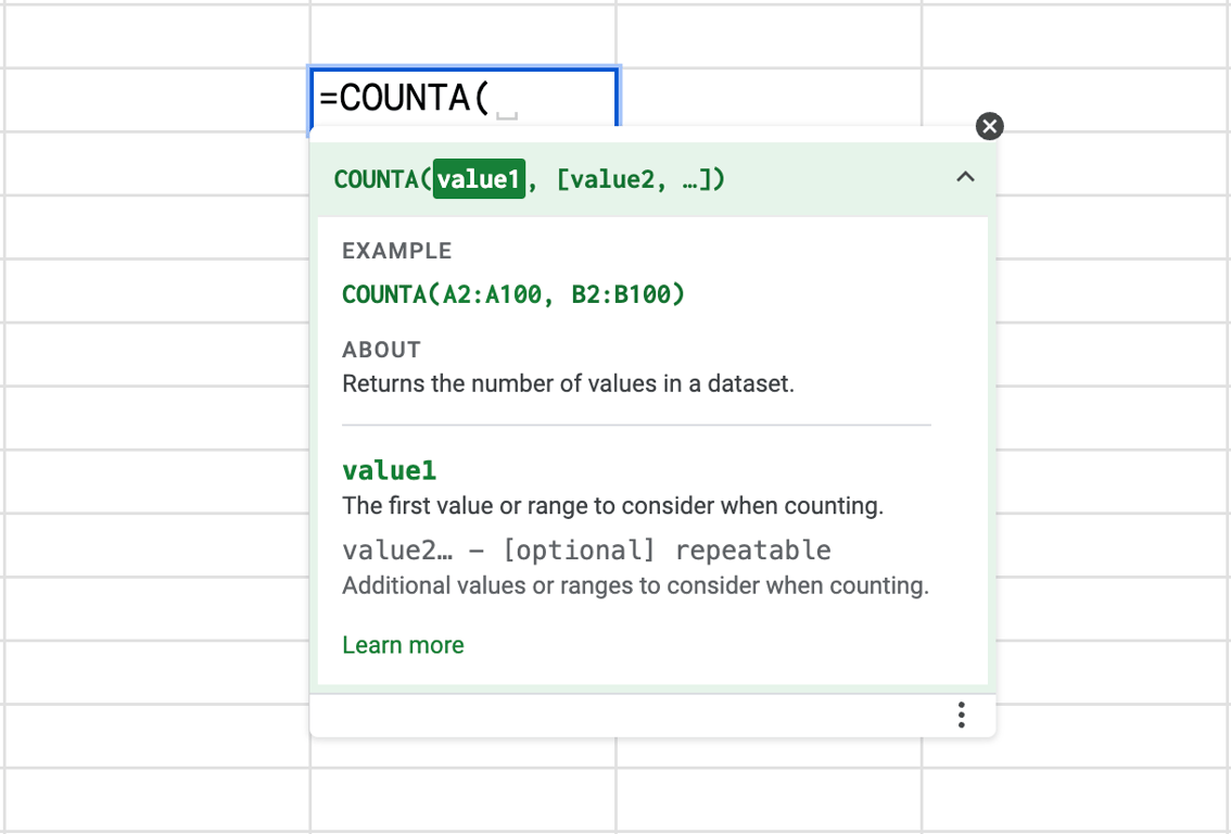
COUNTA counts the non-empty cells of what UNIQUE returns, which gives the number of distinct values:
=COUNTA(UNIQUE(B3:B15))
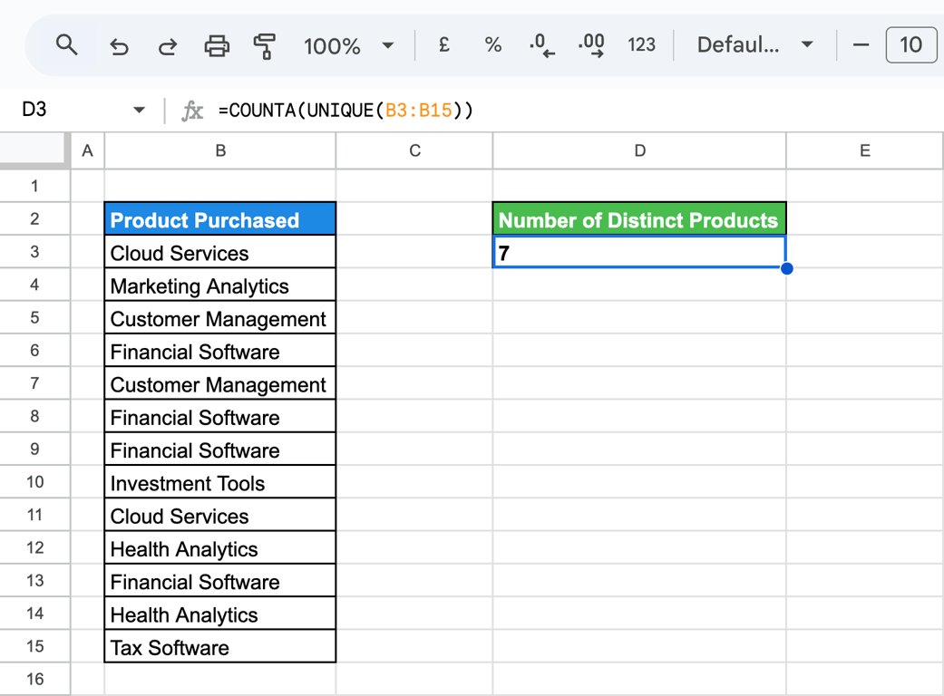
=COUNTUNIQUE(B3:B15) returns the same number in one function.
UNIQUE and SORT: distinct rows in order
=SORT(UNIQUE(B3:C15))
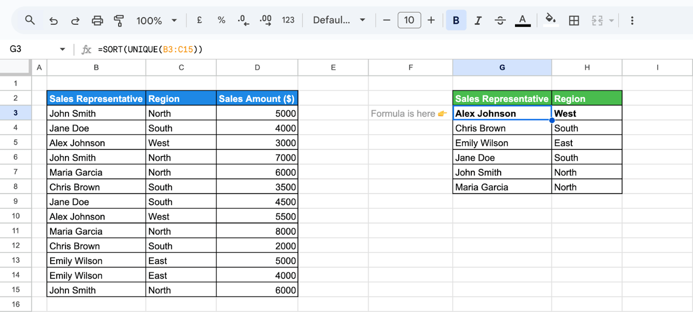
The duplicate rows are removed first, then the result is sorted by the first column.
UNIQUE and FILTER: distinct values that meet a condition
FILTER narrows the range before UNIQUE sees it:
=SORT(UNIQUE(FILTER(B3:B15, C3:C15 > 100)))
This returns, in alphabetical order, each value of column B whose row has more than 100 in column C. The same pattern removes the blank entry that UNIQUE returns when the range contains empty cells: =UNIQUE(FILTER(B3:B15, B3:B15 <> "")).
UNIQUE and QUERY: distinct values from a query result
The query language of the QUERY function has no DISTINCT keyword, so wrap the query in UNIQUE. To list each customer who made a purchase on January 15, 2023:
=UNIQUE(QUERY(B3:C15, "select B where C = date '2023-01-15'"))
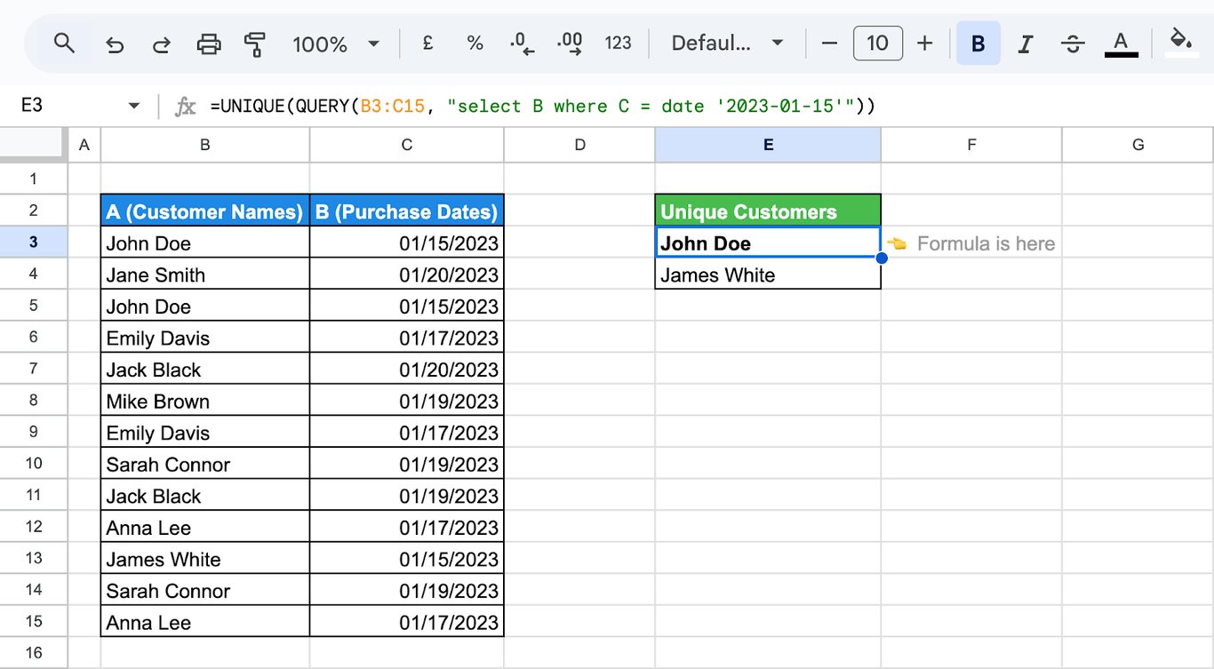
- QUERY(…): returns the customer names (column B) whose purchase date (column C) is 2023-01-15.
- UNIQUE(…): removes the repeated names.
💡 More on this combination in QUERY with UNIQUE in Google Sheets.
Why UNIQUE returns values that look like duplicates
Why UNIQUE returns values that look like duplicates
UNIQUE compares the cell contents exactly. Two cells that look the same to you can still differ.
Different capitalization
⚠️ Issue: “Apple” and “apple” are returned as two values.
✅ Solution: Standardize the case first: =UNIQUE(ARRAYFORMULA(LOWER(B3:B15))).
Extra spaces
⚠️ Issue: “Apple” and “Apple “ (with a trailing space) are two values.
✅ Solution: Remove the spaces with TRIM: =UNIQUE(ARRAYFORMULA(TRIM(B3:B15))).
Numbers stored as text
⚠️ Issue: The number 100 and the text “100” are two values.
✅ Solution: Convert the column to one type, with VALUE for numbers or TO_TEXT for text, before applying UNIQUE.
An empty row in the result
⚠️ Issue: If the range contains empty cells, the result includes one empty entry.
✅ Solution: Filter them out: =UNIQUE(FILTER(B3:B15, B3:B15 <> "")).
Merged cells
⚠️ Issue: A merged cell holds its value in the top left cell only; the rest of the merged area is empty. UNIQUE then returns the value and an empty entry.
✅ Solution: Unmerge the cells (Format → Merge cells → Unmerge) and fill in the values.
Errors in the UNIQUE function
#REF!: the result has no room
The most common error. UNIQUE needs empty cells for its result. If any of them contains data, the formula returns #REF!, and hovering over it names the cell that is in the way. Clear the cells below and to the right of the formula.
#REF! also appears when the formula points to a tab that does not exist, for example after the tab was renamed or deleted:
=UNIQUE(Sheet8!B3:E15)
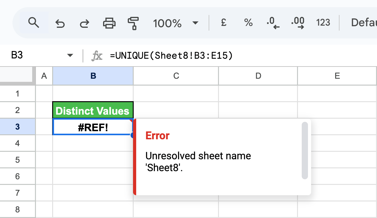
Correct the tab name in the formula.
#VALUE!: the argument is not a range
=UNIQUE("Customer Names and Purchase Dates!", "B2:B200")
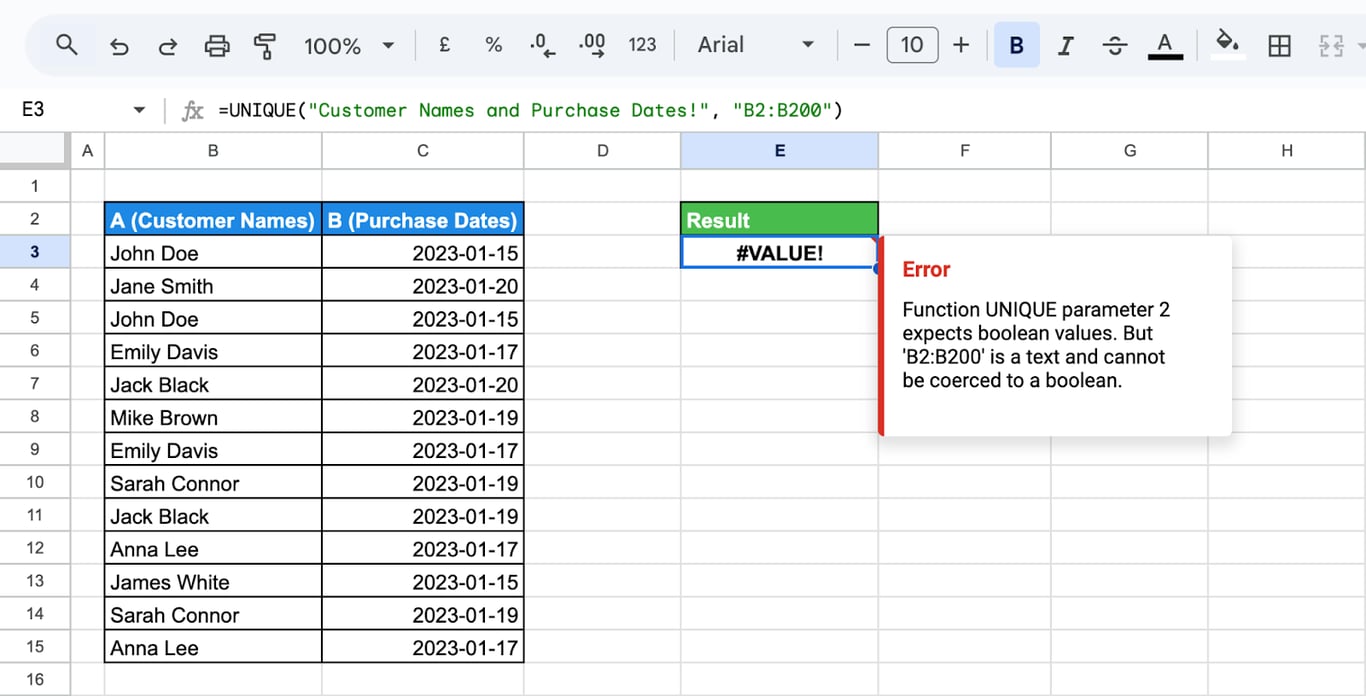
Here the range was typed as two pieces of text. UNIQUE needs a range reference, written without quotes: =UNIQUE(B2:B200).
#N/A: the range is missing
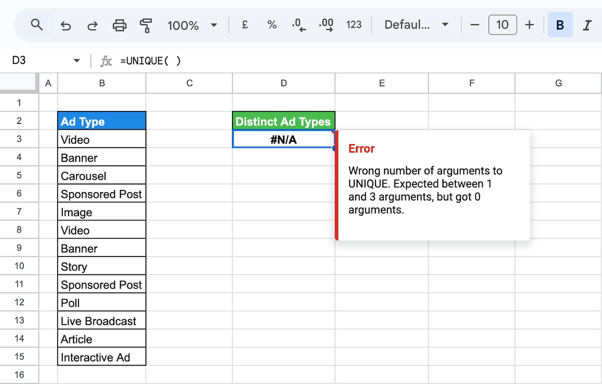
UNIQUE with no range, or with the wrong number of arguments, returns #N/A. Add the range.
#NAME?: the function name is misspelled
=UNIQE(B3:B15)
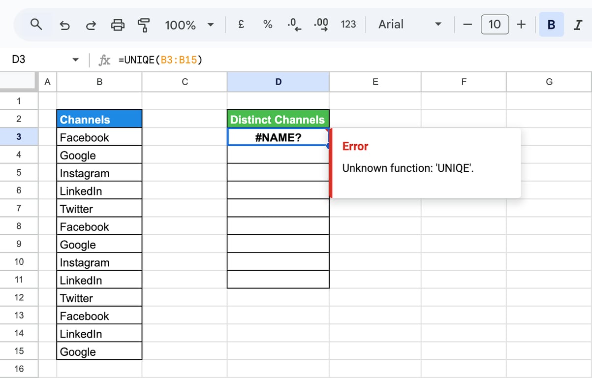
Google Sheets does not know a function called UNIQE. Correct the spelling to =UNIQUE(B3:B15).
Related Google Sheets functions
Related Google Sheets functions
Functions that are often used next to UNIQUE, each with its own guide:
- VLOOKUP: Searches the first column of a range and returns a value from the same row.
- XLOOKUP: A more flexible lookup that can return values from any direction.
- MATCH: Returns the relative position of an item in a range.
- CONCATENATE: Joins several pieces of text into one string.
- FILTER: Returns the rows of a range that meet your conditions.
- IMPORTRANGE: Imports a range from another spreadsheet.
UNIQUE removes duplicates, it cannot say why they are there
UNIQUE removes duplicates, it cannot say why they are there
A list with duplicates has usually been assembled by hand: two exports pasted under each other, a tab copied from last month, a join done with VLOOKUP that matched a customer twice. UNIQUE cleans up the symptom every time the sheet is opened. It cannot tell you whether the duplicated orders were also counted twice in the revenue column next to them.
The OWOX Data Marts extension for Google Sheets covers that half. A data analyst publishes a data mart (a table or an SQL query in your data warehouse) and makes it available for reports. In Sheets you open the extension, pick the data mart, tick the columns you want and run it. The rows land in a tab, ready for your formulas.
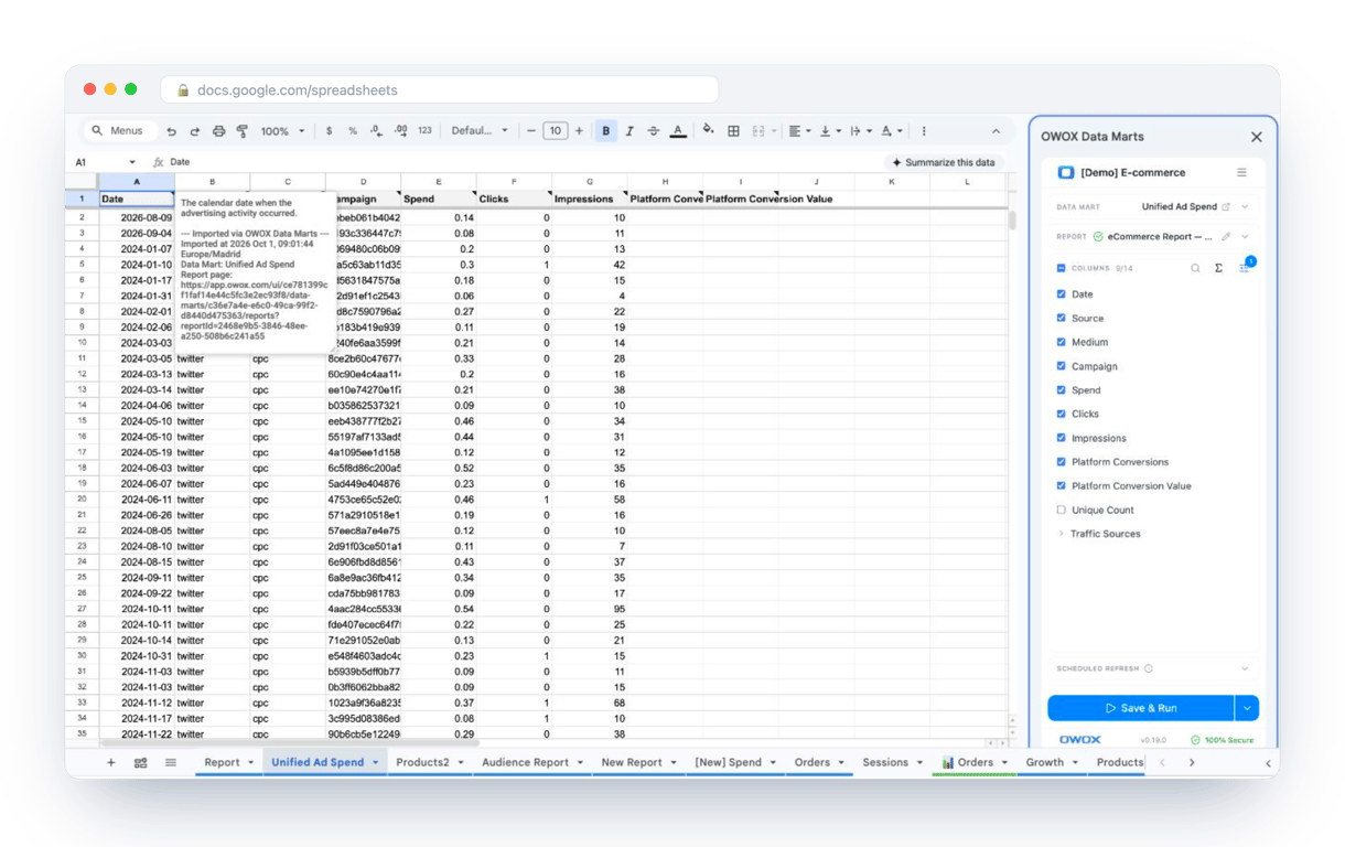
What changes for the person who maintains the sheet:
- Refresh replaces re-export. Refresh current report in the extension menu re-runs the same pull, and a scheduled refresh keeps the tab current without anyone touching it.
- The source is written on the sheet. The header cell of an imported tab carries a note with the data mart it came from, the time of the import and a link to the report.
- No SQL and no warehouse access needed. The analyst decides which data marts and columns are available. You choose from that list.
The extension does not write or change the analyst’s SQL: whether an order appears once is decided there, in one place, and UNIQUE goes back to its real job of listing the distinct values in a column. The extension comes with the OWOX Cloud plans of OWOX Data Marts; spreadsheet reporting describes both ways data reaches a sheet.
Turn your data into decisions.
Governed data marts give you the clean foundation ML needs to actually work.
- No AI hallucinations
- Analyst-governed definitions
- Every number traces to SQL
Frequently Asked Questions
Why is my UNIQUE formula not working?
If your UNIQUE formula isn't working, check for empty rows/columns in your range, ensure the range is correctly specified, and verify that your data doesn't contain subtle duplicates.
How do I get unique (or distinct) values from another sheet in Google Sheets?
To get distinct values from another sheet in Google Sheets, use =UNIQUE(SheetName!range), replacing 'SheetName' and 'range' with the relevant sheet name and cell range. If you want to get a list of unique values you need to add the second parameter and set it to TRUE as in =UNIQUE(SheetName!range, , TRUE), so it will return only those values that appear exactly once in the range – what is identified as unique values.
How do I use COUNTA with UNIQUE?
Use =COUNTA(UNIQUE(range)). UNIQUE returns each distinct value once and COUNTA counts them, so the result is the number of distinct values in the range. =COUNTUNIQUE(range) returns the same number with one function.
How to extract distinct values based on criteria in Google Sheets?
To extract distinct values based on criteria, combine UNIQUE with FILTER: =UNIQUE(FILTER(range, criteria_range=criteria)), specifying your range, criteria range, and criteria.
How to do a unique query in Google Sheets?
The query language of the QUERY function has no DISTINCT keyword. Wrap the query in UNIQUE instead: =UNIQUE(QUERY(range, "select B where C > 100")). For one row per group with totals, use group by inside the query.
How do you use the UNIQUE function in Google Sheets?
To use the UNIQUE function in Google Sheets, simply type =UNIQUE(range) where 'range' is the cell range you want to extract distinct values from.