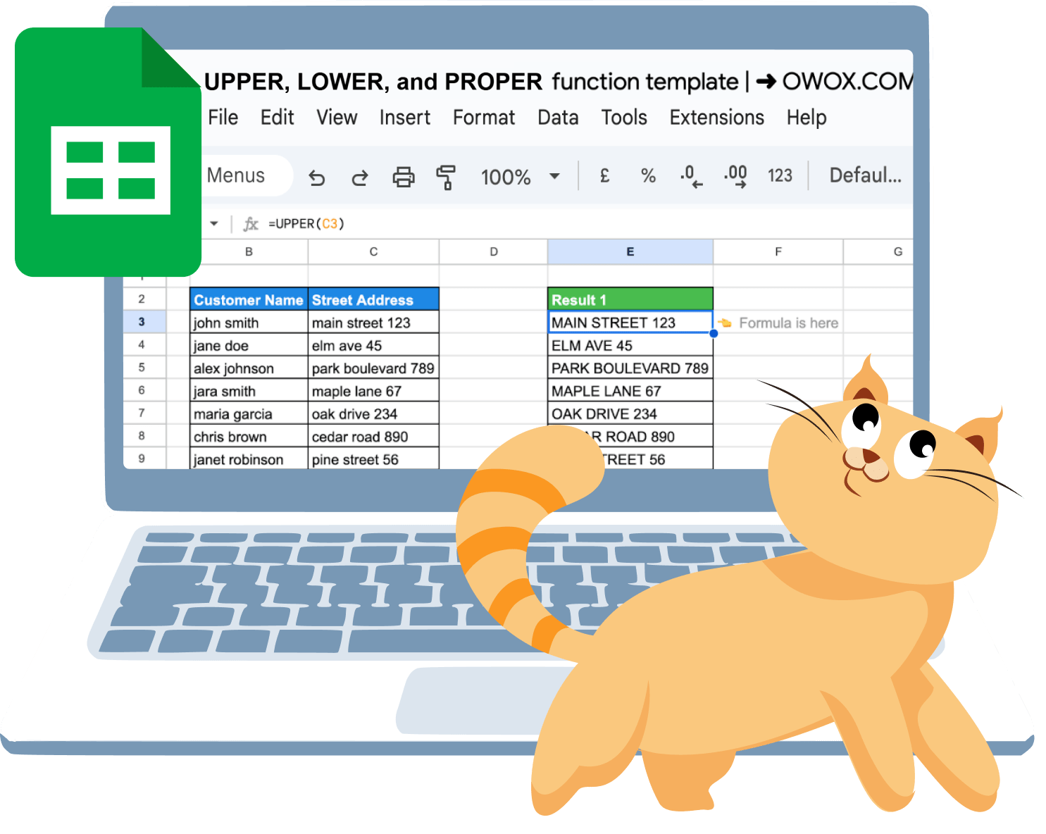
Master Case Conversion in Google Sheets with UPPER, LOWER, and PROPER Functions

Consistent text formatting is essential for maintaining clean, professional-looking data in Google Sheets. The UPPER, LOWER, and PROPER functions provide an easy way to convert text to uppercase, lowercase, or title case, ensuring uniformity across datasets.

Whether you're standardizing names, formatting product listings, or cleaning up imported data, these functions can save time and reduce manual errors. This guide will walk you through how each function works, real-world examples of their usage, and tips to enhance your workflow. 

Learn how to master case conversion in Google Sheets and keep your spreadsheets organized and professional.

When to Use UPPER, LOWER, and PROPER Functions in Google Sheets

The UPPER, LOWER, and PROPER functions in Google Sheets help standardize text formatting for better readability and consistency. Use UPPER when you need to convert all letters in a text string to uppercase, such as when formatting country codes or making text stand out. 

LOWER is useful for converting text to all lowercase, often applied to email addresses or usernames. PROPER capitalizes the first letter of each word while converting the rest to lowercase, making it ideal for formatting names, titles, or addresses. 

These functions are particularly handy when dealing with inconsistent text data, ensuring a uniform and professional appearance in your spreadsheet.

Understanding UPPER, LOWER, and PROPER Functions: Syntax and Examples

The UPPER, LOWER, and PROPER functions in Google Sheets adjust text capitalization for clarity. UPPER converts text to all caps, LOWER makes it lowercase, and PROPER capitalizes the first letter of each word. These functions help standardize names, titles, and other text for better readability.

UPPER Function 

The UPPER function in Google Sheets converts text to uppercase, making it useful for standardizing formatting and ensuring consistency in data entry. It helps highlight important information, such as names, product codes, or headings. 

By applying UPPER, you can quickly transform lowercase or mixed-case text into a uniform, professional format without manual retyping.

Syntax of UPPER

The UPPER function in Google Sheets converts all letters in a given text string to uppercase. 

Its syntax is:

=UPPER(text)

The function requires an argument:

• text: The text you want converted to uppercase. It can be a direct string (e.g., "hello") or a cell reference (e.g., A1).

This function is useful for standardizing text formatting, ensuring consistency in names, headings, and other data entries.

Example of UPPER

The UPPER function is useful when you need to convert text to uppercase for consistency. Suppose you have a list of customer names in lowercase and want to standardize them in uppercase.

To achieve this, use the formula:

=UPPER(B3)

Here’s the breakdown:

• UPPER: Converts all lowercase letters in a text string to uppercase.
• B3: The function takes the value in cell B3 as input.

This function ensures uniformity in data formatting, making it ideal for database records, name standardization, and professional documents.

LOWER Function

The LOWER function in Google Sheets converts all uppercase letters in a text string to lowercase. It is useful for standardizing text, ensuring consistency in names, email addresses, and other data entries. By applying this function, you can quickly format text without manually retyping, improving readability and data accuracy.

Syntax of LOWER

The LOWER function in Google Sheets converts all uppercase letters in a text string to lowercase. 

Its syntax is:

=LOWER(text)

The function requires an argument:

• text: The string to convert to lowercase. The text argument can be a direct string (e.g., "HELLO") or a cell reference (e.g., A1).

This function is useful for standardizing text formatting in datasets.

Example of LOWER

The LOWER function is useful for standardizing text by converting all uppercase letters to lowercase. This is helpful when formatting names, email addresses, or other text entries for consistency.

To achieve this, use the formula:

=LOWER(B3)

Here’s the breakdown:

• LOWER: Converts all uppercase letters in a text string to lowercase.
• B3: The function takes the value in cell B3 as input.

This function is especially useful when working with databases, ensuring uniform text formatting and avoiding inconsistencies in case-sensitive applications.

PROPER Function

The PROPER function in Google Sheets capitalizes the first letter of each word in a text string while converting the rest to lowercase. It is useful for formatting names, titles, and addresses to ensure proper capitalization. This function helps improve data consistency and readability by automatically correcting improper letter casing.

Syntax of PROPER

The PROPER function in Google Sheets capitalizes the first letter of each word while converting the rest to lowercase. 

Its syntax is:

=PROPER(text_to_capitalize)

The function requires an argument:

• text_to_capitalize: The text, which will be returned with the first letter of each word in uppercase and all other letters in lowercase.

The text_to_capitalize argument can be a direct string (e.g., "hello world") or a cell reference (e.g., A1). This function is useful for formatting names and titles consistently.

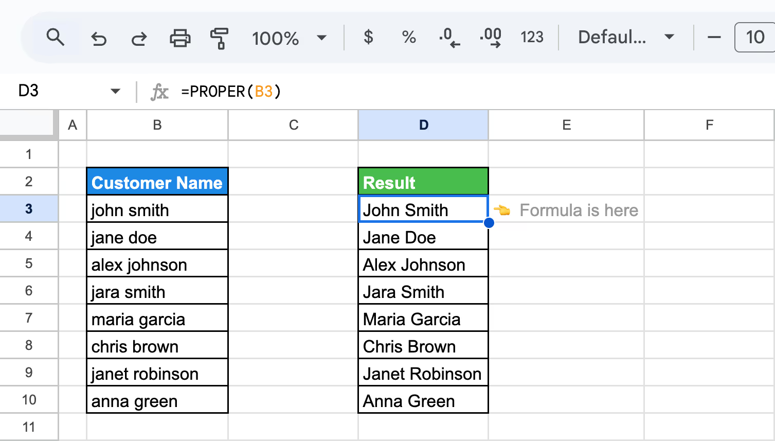
Example of PROPER

The PROPER function is useful for formatting text by capitalizing the first letter of each word while converting the rest to lowercase. This is helpful when standardizing names, addresses, or titles for consistency.

To achieve this, use the formula:

=PROPER(B3)

Here’s the breakdown:

• PROPER: Capitalizes the first letter of each word while converting the rest to lowercase.
• B3: The function takes the value in cell B3 as input.

This function is ideal for formatting customer names, database records, and formal documents for improved readability and consistency.

Master Case Conversion with Our UPPER, LOWER, and PROPER Template!

Practice every example from the article with this ready-to-use template. Download it now and start converting text case effortlessly in Google Sheets.

Get your FREE template now!

Practical Applications of UPPER, LOWER, and PROPER Functions in Google Sheets

The UPPER, LOWER, and PROPER functions in Google Sheets help standardize text formatting for consistency and readability. They are useful for formatting names, correcting capitalization errors, standardizing email addresses, and ensuring uniform text.

In the following examples, we’ll use a unified customer sales dataset to show how each function can be applied to real-world fields like names, email addresses, and street addresses.

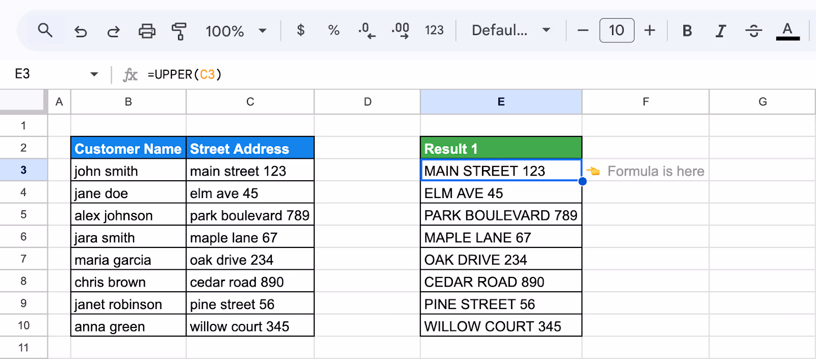
Capitalizing Text in Strings with Both Letters and Numbers with UPPER

The UPPER function in Google Sheets is useful for converting text to uppercase, even when it contains both letters and numbers. This ensures consistency in formatting, especially for product codes, serial numbers, or mixed-case data.

You can apply the UPPER function to a single cell containing a mix of text and numbers.

Let's use the formula:

=UPPER(C3)

Here’s the breakdown:

• C3: Refers to the Street Address.

Instead of applying the formula to each row individually, you can capitalize an entire range at once using ARRAYFORMULA.

Let's use the formula:

=ARRAYFORMULA(UPPER(C3:C10))

Here’s the breakdown:

• C3:C10: Refers to the range of cells containing text that needs to be converted to uppercase.
• UPPER(): Converts all text within the specified range to uppercase, ensuring uniform formatting.
• ARRAYFORMULA: Allows the UPPER function to be applied to multiple rows at once.

Using UPPER in these ways helps maintain uniform formatting across datasets, improving data accuracy and presentation.

Using LOWER for Converting Email Address Case

The LOWER function in Google Sheets is useful for ensuring consistency in email addresses by converting all letters to lowercase. Since email addresses are not case-sensitive, using LOWER prevents formatting issues and ensures uniformity across datasets.

Let's use the formula:

=LOWER(C3)

Here’s the breakdown:

• C3: Refers to the cell containing the text to be converted to lowercase.
• LOWER(): Converts all uppercase letters in the text within C3 to lowercase, ensuring consistency in formatting.

This method is particularly useful in databases, CRM systems, or sign-up forms where email addresses need to be consistently formatted for accurate processing and validation.

Applying the PROPER Function to an Entire Range for Text Formatting

The PROPER function in Google Sheets is useful for capitalizing the first letter of each word while converting the rest to lowercase. When applied to an entire range, it ensures consistent formatting across multiple entries, such as names, addresses, or job titles.

Let's use the formula:

=ARRAYFORMULA(PROPER(B3:B10))

Here’s the breakdown:

• B3:B10: Refers to the range of cells containing text that needs to be formatted.
• PROPER(): Capitalizes the first letter of each word while converting all other letters to lowercase.
• ARRAYFORMULA: Allows the PROPER function to be applied to multiple rows at once.

Using the PROPER function for bulk formatting saves time and eliminates inconsistencies in large datasets.

Combining UPPER, LOWER, and PROPER with Other Functions in Google Sheets

Combining UPPER, LOWER, and PROPER with other functions in Google Sheets enhances text formatting and data processing. These functions can be used alongside formulas that clean, merge, or extract text, ensuring consistent capitalization.

In the following examples, we’ll continue using the same unified customer sales dataset to demonstrate how these case functions work effectively when combined with tools like CONCATENATE, IF, ARRAYFORMULA, and more.

Using CONCATENATE and UPPER to Format Full Names in Uppercase

Combining the UPPER and CONCATENATE functions in Google Sheets allows you to format full names in uppercase while merging first and last names. This ensures uniform formatting, especially in databases or official documents where capitalization consistency is required.

Let's use the formula:

=UPPER(CONCATENATE(B3, " ", C3))

Here’s the breakdown:

• B3: Refers to the first name.
• " ": Adds a space between the first and last name to ensure proper formatting.
• C3: Refers to the last name.
• CONCATENATE(B3, " ", C3): Joins the first name and last name into a single full name string.
• UPPER(): Converts the entire concatenated name into uppercase letters for consistency.

Using UPPER with CONCATENATE simplifies formatting tasks and ensures professional, consistent text presentation.

Using UPPER with IF for Conditional Formatting

Combining the UPPER function with IF in Google Sheets allows you to apply conditional formatting based on specific criteria. For example, you can use it to automatically convert text to uppercase when a certain condition is met, such as marking VIP customers or highlighting priority tasks.

Let's use the formula:

=IF(C3="VIP", UPPER(B3), B3)

Here’s the breakdown:

• C3: Refers to the status of the customer.
• "VIP": The condition being checked – if C3 contains "VIP", the formula applies the next step.
• UPPER(B3): If C3 equals "VIP", the function converts the name in B3 to uppercase for emphasis.
• B3: If C3 is not "VIP", the name remains unchanged.
• IF(): Evaluates the condition and determines whether to apply the uppercase transformation or leave the text as is.

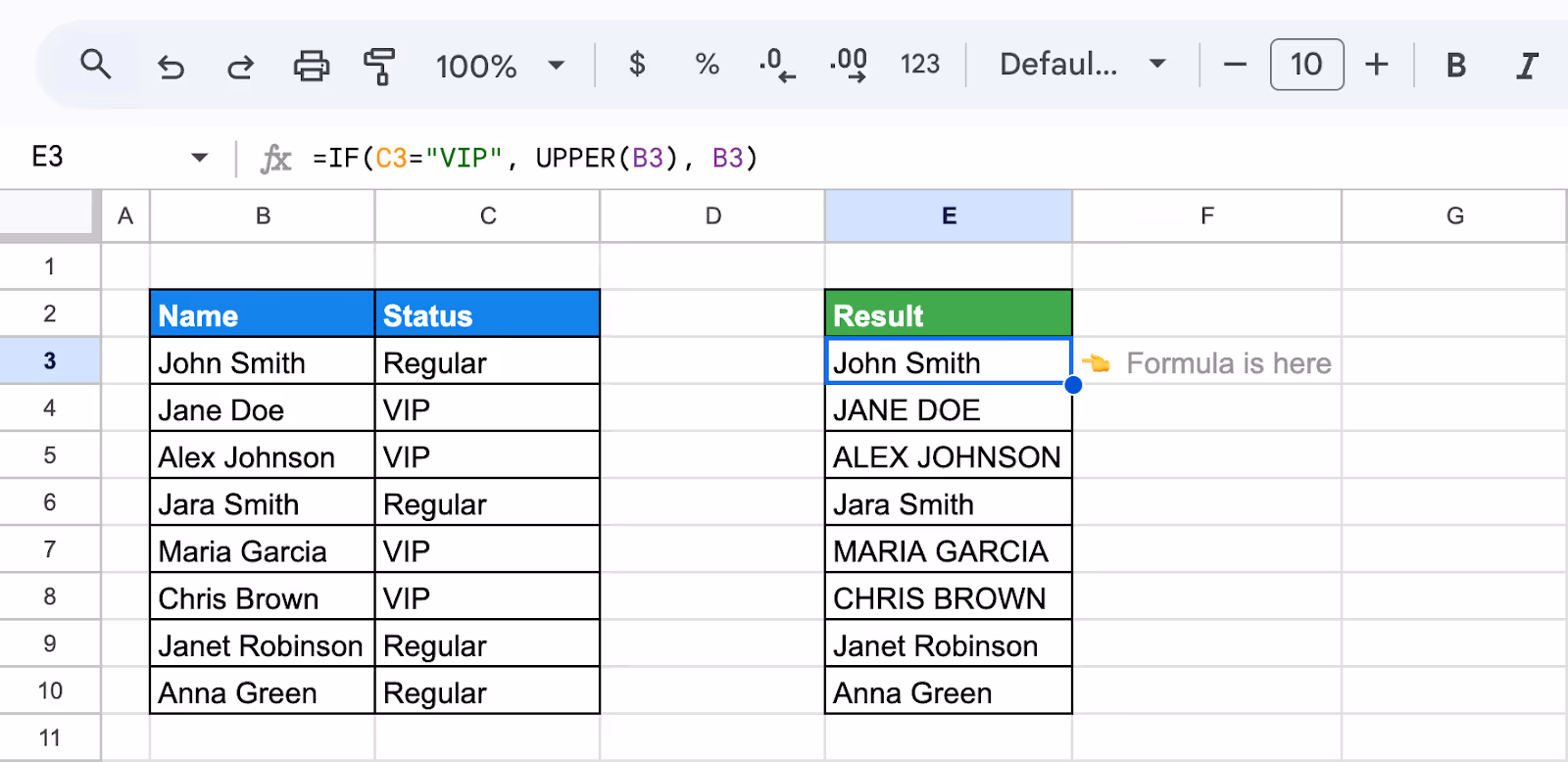
This method ensures that important names or priority items stand out, making data more readable and organized for reports or customer management systems.

Using LOWER with ARRAYFORMULA to Convert Text to Lowercase

The LOWER function in Google Sheets is useful for converting text to lowercase, ensuring consistency in data formatting. When combined with ARRAYFORMULA, it applies the transformation to an entire range at once, eliminating the need to manually copy the formula down.

Let's use the formula:

=ARRAYFORMULA(LOWER(C3:C10))

Here’s the breakdown:

• C3:C10: Refers to the range of cells containing text that needs to be converted to lowercase.
• LOWER(): Converts all uppercase letters in the specified range to lowercase, ensuring uniform text formatting.
• ARRAYFORMULA: Enables the LOWER function to process multiple rows at once.

This method is especially useful for standardizing email addresses, usernames, or any text that requires a uniform lowercase format across large datasets.

Using LOWER with LEFT, RIGHT, or MID for Specific Text Formatting

Combining the LOWER function with LEFT, RIGHT, or MID in Google Sheets allows for extracting and formatting specific parts of text. This is useful for standardizing product codes, abbreviating location names, or modifying data for easier categorization.

The LEFT function extracts the first few characters from a text string. When combined with LOWER, it ensures the extracted portion is in lowercase.

Let's use the formula:

=LOWER(LEFT(C3,3))

Here’s the breakdown:

• C3: Refers to the original text value from which characters will be extracted.
• LEFT(C3,3): Extracts the first 3 characters from the text in C3.
• LOWER(): Converts the extracted portion to lowercase.

The MID function extracts text from a specific position within a string. Combined with LOWER, it converts the extracted portion into lowercase.

Let's use the formula:

=LOWER(MID(C3,3,3))

Here’s the breakdown:

• C3: Refers to the original text value from which characters will be extracted.
• MID(C3,3,3): Extracts 3 characters starting from the third position in C3.
• LOWER(): Converts the extracted portion to lowercase.

The RIGHT function extracts the last few characters from a text string. Combined with LOWER, it ensures the extracted portion is lowercase.

Let's use the formula:

=LOWER(RIGHT(C3,3))

Here’s the breakdown:

• C3: Refers to the original text value from which characters will be extracted.
• RIGHT(C3,3): Extracts the last 3 characters from the text in C3.
• LOWER(): Converts the extracted portion to lowercase.

These examples demonstrate how combining LOWER with LEFT, MID, or RIGHT helps standardize text formatting, making it useful for abbreviations, categorization, or short-code generation.

Using UPPER, LOWER, LEFT, RIGHT, and LEN Functions to Capitalize Only the First Letter of a Sentence

In Google Sheets, you can capitalize only the first letter of a sentence while keeping the rest in lowercase by combining UPPER, LOWER, LEFT, RIGHT, and LEN functions. This is useful for standardizing text formatting in sentences, product descriptions, or names while ensuring proper capitalization.

Let's use the formula:

=UPPER(LEFT(C3,1))&LOWER(RIGHT(C3,LEN(C3)-1))

Here’s the breakdown:

• C3: Refers to the text string (sentence) that needs to be formatted.
• LEFT(C3,1): Extracts the first character from the text in C3.
• UPPER(LEFT(C3,1)): Converts the extracted first letter to uppercase.
• LEN(C3): Calculates the total number of characters in C3.
• RIGHT(C3, LEN(C3)-1): Extracts all characters except the first one (i.e., from the second character onward).
• LOWER(RIGHT(C3, LEN(C3)-1)): Converts the extracted text (everything except the first letter) to lowercase.
• &: Joins the capitalized first letter with the rest of the lowercase text, forming a properly formatted sentence.

This approach ensures consistent sentence formatting, making text look clean and professional.

Using the PROPER and TRIM functions to Clean and Format Text

When working with messy or improperly formatted text, combining PROPER and TRIM in Google Sheets helps clean up inconsistencies. PROPER capitalizes the first letter of each word, while TRIM removes extra spaces, ensuring text is well-formatted and easy to read. This is particularly useful for cleaning up names, job titles, or addresses.

Let's use the formula:

=PROPER(TRIM(C3))

Here’s the breakdown:

• C3: Refers to the text string that needs to be cleaned and formatted.
• TRIM(C3): Removes any extra spaces before, after, and between words, leaving only single spaces.
• PROPER(TRIM(C3)): Capitalizes the first letter of each word while converting the rest of the text to lowercase.

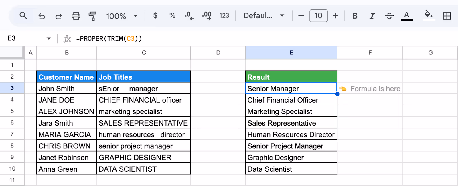
This approach is especially useful when dealing with imported data, fixing errors in large datasets, or ensuring standardized formatting across documents.

Using PROPER and CONCATENATE to Standardize Full Names

In Google Sheets, combining PROPER with CONCATENATE ensures that full names are correctly formatted with proper capitalization. PROPER capitalizes the first letter of each word, while CONCATENATE merges first and last names into a single formatted entry. This is useful for cleaning up name lists in databases, forms, or reports.

Let's use the formula:

=PROPER(CONCATENATE(B3, " ", C3))

Here’s the breakdown:

• B3: Refers to the first name, which may have inconsistent capitalization.
• " ": Adds a space between the first and last name to ensure proper formatting.
• C3: Refers to the last name, which may also have inconsistent capitalization.
• CONCATENATE(B3, " ", C3): Joins the first and last names into a single string with a space in between.
• PROPER(CONCATENATE(B3, " ", C3)): Ensures that the first letter of each word is capitalized while converting the rest of the text to lowercase.

This formula is useful for standardizing full names in databases, contact lists, or official documents, ensuring proper capitalization and consistency.

Troubleshooting Common Errors with UPPER, LOWER, and PROPER Functions

When using UPPER, LOWER, and PROPER functions in Google Sheets, errors may occur due to unexpected spaces, special characters, or formatting issues. These functions only work with text, so numbers remain unchanged. Ensuring clean and consistent data can help prevent common problems and improve accuracy.

Mixed Text and Number Errors

⚠️ Error: The PROPER function may not format text correctly when a cell contains a mix of text and numbers. It only capitalizes letters while leaving numbers unchanged, which can result in inconsistent formatting, especially when dealing with product codes, addresses, or mixed alphanumeric entries.

✅ Solution: If you need uniform formatting, consider separating text and numbers into different cells before applying PROPER. Alternatively, use functions like TEXT() to format numbers as text where necessary. Always check data consistency to ensure the function produces the desired results.

Error with Apostrophes and Special Characters

⚠️ Error: The PROPER function may not handle apostrophes and special characters correctly. It can misplace capitalization in words with apostrophes, like "O'Connor," or struggle with special characters, leading to inconsistent formatting. This can be problematic when dealing with names, brand titles, or text with punctuation.

✅ Solution: Manually review and adjust text formatting for cases where PROPER does not work as expected. If needed, use SUBSTITUTE() to replace problematic characters or apply TEXT() to maintain the correct format. For names or proper nouns, verify capitalization manually to ensure accuracy.

Nesting Functions Improperly

⚠️ Error: The UPPER function may not work correctly if nested improperly within other functions. For example, using UPPER inside a formula that expects a number, such as SUM(UPPER(A1:A10)), can cause errors. Additionally, applying it to non-text values or functions that return numbers can lead to unexpected results.

✅ Solution: Ensure that UPPER is only applied to text-based data. If working with mixed content, use TEXT() to convert numbers into strings before applying UPPER. When nesting functions, verify that each function outputs the expected data type to avoid errors.

#VALUE!

⚠️ Error: The #VALUE! error occurs in the PROPER and LOWER functions when they reference invalid data types, such as formula errors or non-text values that cannot be processed. This issue often arises when the function is applied to cells containing errors like #N/A, #REF!, or numbers formatted in a way that the function cannot interpret as text.

✅ Solution: Check all referenced cells for errors or incompatible data. If numbers need to be included, convert them to text using the TEXT() function before applying PROPER or LOWER. Additionally, use IFERROR() to handle problematic values and ensure the function operates smoothly.

#NAME?

⚠️ Error: The #NAME? error occurs in the UPPER, PROPER, and LOWER functions when there is a typo in the function name, missing quotation marks around text, or an undefined reference. This typically happens if the function name is misspelled or if a referenced cell or range does not exist.

✅ Solution: Double-check the function name for spelling errors and ensure that all text inputs are enclosed in quotation marks. Verify that referenced cells exist and are correctly formatted. If using named ranges, confirm they are defined correctly in the spreadsheet.

#ERROR!

⚠️ Error: The #ERROR! message appears in the UPPER, PROPER, and LOWER functions when Google Sheets encounters a formula structure issue. This can happen if there are missing parentheses, incorrect argument types, or improperly combined functions. The error indicates that the formula cannot be interpreted correctly.

✅ Solution: Review the formula structure to ensure correct syntax. Check that all parentheses are properly closed and that the function is applied to valid text values. If nesting functions, verify that each function returns the expected data type. Testing with a simple text input can help identify the source of the issue.

#REF!

⚠️ Error: The #REF! error occurs in the UPPER, PROPER, and LOWER functions when the formula references an invalid or deleted cell. This typically happens if a referenced cell is removed or if the function attempts to use a non-existent range, leading to broken references.

✅ Solution: Check for deleted or missing cells in the formula and restore any necessary references. If pasting new data over existing references, ensure formulas are updated accordingly. Using IFERROR() can help handle missing data gracefully, preventing formula breakage when references change.

Best Ways to Use UPPER, LOWER, and PROPER Functions in Google Sheets

The UPPER, LOWER, and PROPER functions in Google Sheets are useful for adjusting text capitalization. They help standardize formatting, improve readability, and ensure consistency in data. Whether converting text to all caps, lowercase, or proper case, these functions make it easier to organize and present information clearly.

Create a Duplicate Sheet Before Text Manipulation

Before using the UPPER, PROPER, or LOWER functions in Google Sheets, it's a good practice to create a duplicate sheet. This ensures you have a backup in case of errors or unintended changes during text manipulation. Having a copy allows you to compare results and restore original data if needed. 

Leveraging Conditional Formatting with Text Functions

Using UPPER, PROPER, and LOWER functions with conditional formatting in Google Sheets helps highlight inconsistencies in text formatting. You can set rules to detect improperly capitalized text, ensuring uniform data presentation.

For example, highlighting cells that aren’t in uppercase or proper case allows for quick corrections, improving data accuracy and consistency across your spreadsheet.

Building a Custom Function for Your Specific Needs

If the LOWER function in Google Sheets doesn’t fully meet your needs, you can build a custom function using Google Apps Script. This allows for more advanced text formatting, such as handling special characters or applying lowercase conversion selectively. Custom functions provide greater flexibility, ensuring text is processed exactly as required for your specific use case.

Using ARRAYFORMULA with Text Functions

Using ARRAYFORMULA with UPPER, PROPER, and LOWER functions in Google Sheets allows you to apply text transformations to an entire column at once. Instead of modifying each cell individually, ARRAYFORMULA automates the process, saving time and ensuring consistency. 

This is especially useful when working with large datasets, making bulk formatting more efficient and reducing manual work.

Using CLEAN and TRIM with the UPPER Function

When using the UPPER function in Google Sheets, combining it with CLEAN and TRIM helps remove unwanted characters and spaces for cleaner results. CLEAN removes non-printable characters, while TRIM eliminates extra spaces, ensuring text is properly formatted before converting it to uppercase. This combination improves data accuracy and prevents formatting issues in large datasets.

Power Up Your Spreadsheet Workflow with These Key Google Sheets Functions

Google Sheets provides powerful formulas that help automate workflows, clean up data, and extract deeper insights with less manual effort.

• REGEX: Enable pattern-based searching, extraction, and replacement in text data, making them ideal for data cleaning, formatting, and validation tasks.
• VLOOKUP: Searches for a value in the first column of a range and returns a value in the same row from a specified column, useful for pulling related data across tables.
• IMPORTRANGE: Imports a range of cells from a different Google Sheets document, enabling seamless cross-sheet data integration for centralized reporting.
• COUNTA: Counts the number of non-empty cells in a range, helping quickly assess the volume of entries without filtering or sorting.
• MATCH: Finds the relative position of a specified value in a range, aiding lookup operations and position-based logic for dynamic formulas.
• QUERY: Performs complex data manipulations using SQL-like syntax, allowing advanced filtering, sorting, grouping, and pivoting — all within your spreadsheet.

Simplify Your Data Visualization with OWOX: Reports, Charts & Pivots Extension

Case conversion functions like UPPER, LOWER, and PROPER make formatting text easier, but manually adjusting large datasets can be time-consuming. OWOX: Reports, Charts & Pivots Extension helps you automate repetitive tasks, generate insightful reports, and visualize data with ease. 

Whether you're cleaning up text or streamlining workflows, OWOX saves you time and effort. Install the OWOX Reports Extension today and take your data efficiency to the next level!