How to use VLOOKUP with an IF statement in Google Sheets
IF and VLOOKUP combine in two ways: IF around VLOOKUP tests the value the lookup returns, and IF inside VLOOKUP chooses the table or the column to search. This guide shows both, plus the shortest way to replace #N/A when nothing is found.
IF and VLOOKUP are combined in two ways. IF around VLOOKUP tests the value that the lookup returns:
=IF(VLOOKUP(G2, B3:D11, 3, FALSE) < TIME(10, 0, 0), "Food is ready", "Food is not ready")
IF inside VLOOKUP decides what the lookup searches: which table, or which column.
| You need | Formula |
|---|---|
| A label that depends on the looked-up value | =IF(VLOOKUP(key, range, 3, FALSE) > 100, "High", "Low") |
| Yes or No: is the key in the table? | =IF(ISNA(VLOOKUP(key, range, 1, FALSE)), "No", "Yes") |
| Your own text instead of #N/A | =IFNA(VLOOKUP(key, range, 2, FALSE), "Not found") |
| An empty result while the key cell is empty | =IF(key = "", "", VLOOKUP(key, range, 2, FALSE)) |
| One of two tables, chosen by a cell | =VLOOKUP(key, IF(I2 = "Royal Place", B4:C11, E4:F11), 2, FALSE) |
| One of several columns, chosen by a cell | =VLOOKUP(key, range, IFS(G3 = "Royal Place", 2, G3 = "Food Fort", 3), FALSE) |
The two functions
=VLOOKUP(search_key, range, index, [is_sorted])
- search_key: the value to look for.
- range: the table. The key is searched in its first column.
- index: the number of the column to return, counted from the left of the range.
- is_sorted (optional): FALSE (or 0) for an exact match. Leave it out, or use TRUE, only when the first column is sorted and you want the nearest match.
=IF(logical_expression, value_if_true, value_if_false)
- logical_expression: a test that is either TRUE or FALSE.
- value_if_true, value_if_false: what to return in each case.
Details of each are in the guides to VLOOKUP and the IF function.
IF around VLOOKUP: test the value the lookup returns
IF around VLOOKUP: test the value the lookup returns
Put the whole VLOOKUP into the first argument of IF and compare its result with something. The table lists menu items with the price and the time each order was placed. An order placed before 10:00 AM is ready for pickup:
=IF(VLOOKUP(G2, B3:D11, 3, FALSE) < TIME(10, 0, 0), "Food is ready", "Food is not ready")
- VLOOKUP(G2, B3:D11, 3, FALSE): finds the item named in G2, Pizza, and returns the third column, the time of the order.
- < TIME(10, 0, 0): compares that time with 10:00 AM.
- “Food is ready”, “Food is not ready”: the two possible results.
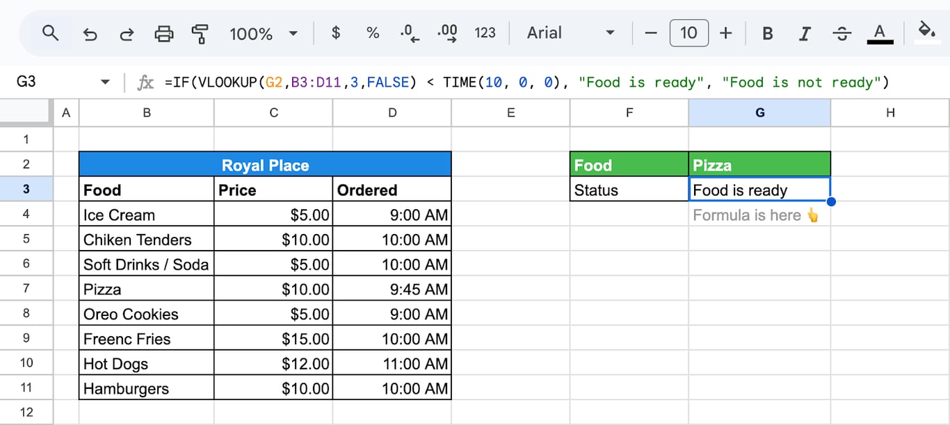
Pizza was ordered at 9:45 AM, so the formula returns “Food is ready”.
Any comparison works here: >, <, >=, <=, = or <>. To compare with text, put the text in quotes: =IF(VLOOKUP(G2, B3:D11, 2, FALSE) = "Sold out", "Remove from menu", "Keep").
OWOX Data Marts
See your first report built in real time. 15 minutes.
- Connect your data warehouse
- Pick your metrics
- Get a live Google Sheets report
In the time it takes to write a ticket. Then imagine never writing that ticket again.
Book a DemoWe'll use your actual use case
IF inside VLOOKUP: choose the table
IF inside VLOOKUP: choose the table
When the same kind of data sits in two tables, IF can hand VLOOKUP the right one. Two restaurants have their price lists side by side, and a cell holds the name of the restaurant to check:
=VLOOKUP(I3, IF(I2 = "Royal Place", B4:C11, E4:F11), 2, 0)
- I3: the item to look up, Hot Dogs.
- IF(I2 = “Royal Place”, B4:C11, E4:F11): if I2 says Royal Place, search its table; otherwise search the table of the other restaurant.
- 2: return the price, the second column of either table.
- 0: exact match.
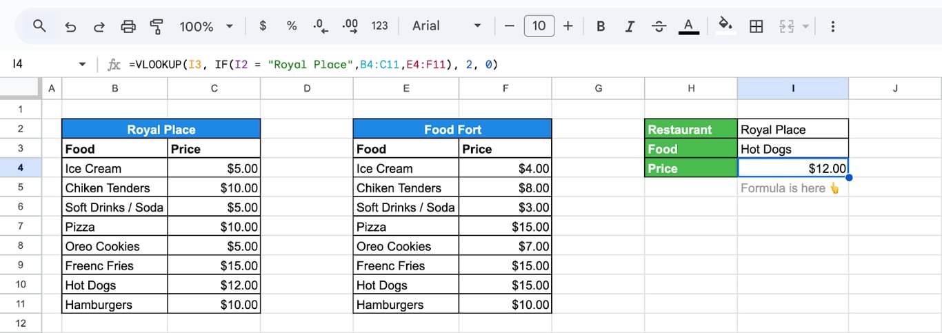
With Royal Place in I2 the formula returns $12.00. Type the other name and it switches to the second table. For three or more tables, replace IF with IFS.
IF inside VLOOKUP: choose the column
IF inside VLOOKUP: choose the column
When the prices of both restaurants are columns of one table, the thing to switch is the column index:
=VLOOKUP(G2, B3:D11, IFS(G3 = "Royal Place", 2, G3 = "Food Fort", 3), 0)
- G2: the item to look up, Oreo Cookies.
- B3:D11: the table: items in the first column, one price column per restaurant.
- IFS(G3 = “Royal Place”, 2, G3 = “Food Fort”, 3): returns 2 or 3 depending on the restaurant named in G3.
- 0: exact match.
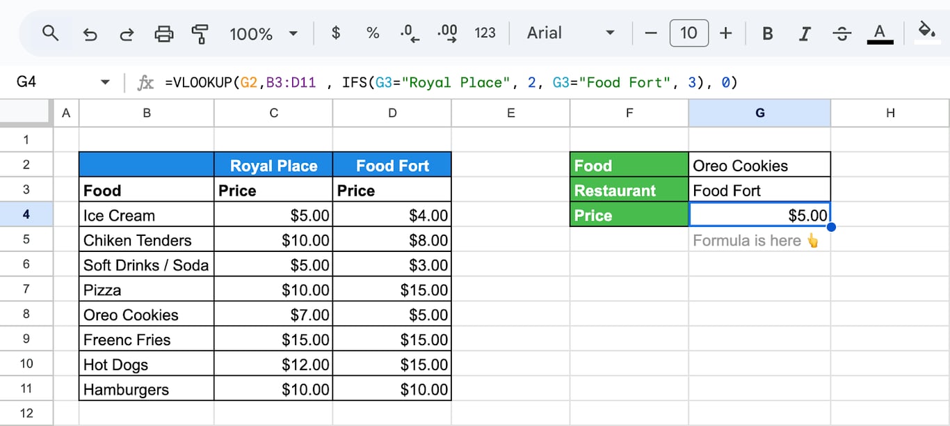
With many columns, MATCH does the same without listing every name: =VLOOKUP(G2, B3:D11, MATCH(G3, B2:D2, 0), 0) finds the position of the restaurant in the header row and uses it as the index.
Replace #N/A when nothing is found
Replace #N/A when nothing is found
VLOOKUP returns #N/A when the key is not in the first column. The long way to replace the error is IF with ISNA, which runs the lookup twice:
=IF(ISNA(VLOOKUP(I3, E3:F11, 2, 0)) = TRUE, "Will be available by 12 PM today", VLOOKUP(I3, E3:F11, 2, 0))
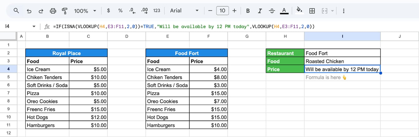
Roasted Chicken is not in the list, so the formula shows the message instead of #N/A.
IFNA does the same in one step:
=IFNA(VLOOKUP(I3, E3:F11, 2, 0), "Will be available by 12 PM today")
IFNA returns the lookup result when there is one and the second argument when the result is #N/A. IFERROR works the same way but hides every kind of error, including a mistyped range, so IFNA is the safer choice.
Keep IF with ISNA for the case where you want different outputs for found and not found: =IF(ISNA(VLOOKUP(I3, E3:F11, 1, 0)), "Not on the menu", "On the menu").
Errors in IF with VLOOKUP formulas
Errors in IF with VLOOKUP formulas
⚠️ Error: #N/A although the key looks the same as the one in the table.
✅ Solution: Look for a trailing space, or a number stored as text on one side. Also check that the key is in the first column of the range: VLOOKUP does not search any other column.
⚠️ Error: A wrong value comes back, with no error.
✅ Solution: The last argument is missing or TRUE. Without FALSE, VLOOKUP assumes that the first column is sorted and returns the nearest match.
⚠️ Error: #REF! in the lookup.
✅ Solution: The index is larger than the number of columns in the range. A range of two columns has no column 3.
⚠️ Error: The comparison is always FALSE.
✅ Solution: The lookup returns text and it is compared with a number, or the other way round. “10” and 10 are different values. Check what the VLOOKUP returns on its own before wrapping it in IF.
⚠️ Error: Formula parse error after copying a formula from a web page.
✅ Solution: The quotes were replaced with typographic ones (“ ”). Retype them as straight quotes.
Related Google Sheets functions
Related Google Sheets functions
Functions that are often used next to IF and VLOOKUP, each with its own guide:
- XLOOKUP: A lookup with a built-in argument for the value to return when nothing is found.
- INDEX and MATCH: A lookup that can return a column to the left of the key.
- VLOOKUP with multiple criteria: Lookups by two or more conditions.
- HLOOKUP: The same lookup across a row.
- ARRAYFORMULA: Runs a lookup for a whole column of keys with one formula.
- QUERY: Filters, sorts and summarizes a table with SQL-like syntax.
- UNIQUE: Returns the distinct values of a range.
Every lookup is a small join
VLOOKUP attaches a value from one table to a row of another, and IF handles the rows where that goes wrong. In a report this is usually a sign that two exports are being matched by hand: orders from one system, prices or names from another. The formula works until a key changes on one side, and then IF quietly prints its fallback text.
The OWOX Data Marts extension for Google Sheets covers that half. A data analyst publishes a data mart (a table or an SQL query in your data warehouse) and makes it available for reports. In Sheets you open the extension, pick the data mart, tick the columns you want and run it. The rows land in a tab, ready for your formulas.
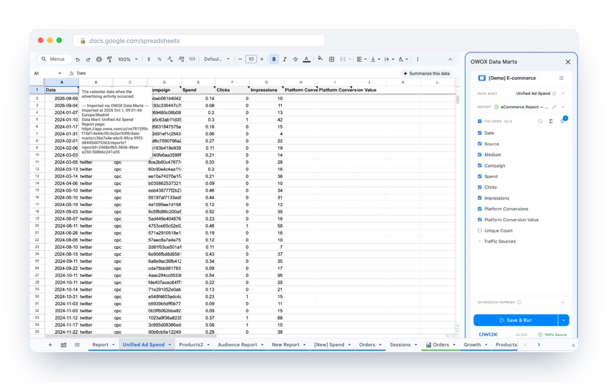
What changes for the person who maintains the sheet:
- Refresh replaces re-export. Refresh current report in the extension menu re-runs the same pull, and a scheduled refresh keeps the tab current without anyone touching it.
- The source is written on the sheet. The header cell of an imported tab carries a note with the data mart it came from, the time of the import and a link to the report.
- No SQL and no warehouse access needed. The analyst decides which data marts and columns are available. You choose from that list.
The extension does not write or change the analyst’s SQL. When the two sources are joined there once, with a real key, the sheet receives the columns already matched, and IF with VLOOKUP goes back to the small lookups that belong in a spreadsheet. The extension comes with the OWOX Cloud plans of OWOX Data Marts; spreadsheet reporting describes both ways data reaches a sheet.
Turn your data into decisions.
Governed data marts give you the clean foundation ML needs to actually work.
- No AI hallucinations
- Analyst-governed definitions
- Every number traces to SQL
Frequently Asked Questions
Are there any limitations or potential issues when combining 'IF' and 'VLOOKUP' in Google Sheets?
Three things to watch. VLOOKUP returns #N/A when the key is missing, so wrap it in IFNA. Without FALSE as the last argument it returns the nearest match, not the exact one. And IF with ISNA runs the lookup twice; IFNA gives the same result with one lookup.
Can you provide an example of when I might need to use 'IF' with 'VLOOKUP' in Google Sheets?
A price list where a cell shows In stock or Out of stock: =IF(VLOOKUP(A2, D:F, 3, FALSE) > 0, "In stock", "Out of stock"), where the third column of the table holds the quantity.
Can this combination be used for more advanced data analysis in Google Sheets?
Yes, it enables conditional data retrieval and analysis in Google Sheets.
What is the syntax for using 'IF' with 'VLOOKUP' in Google Sheets?
IF around VLOOKUP: =IF(VLOOKUP(search_key, range, index, FALSE) = value, value_if_true, value_if_false). IF inside VLOOKUP: =VLOOKUP(search_key, IF(condition, range1, range2), index, FALSE). To replace #N/A: =IFNA(VLOOKUP(search_key, range, index, FALSE), "Not found").
What is the main purpose of combining the 'IF' statement with 'VLOOKUP' in Google Sheets?
It helps control the results of the VLOOKUP based on specific criteria.
How do I combine IF and VLOOKUP together?
In one of two ways. Put VLOOKUP into the logical test of IF to react to the value it returns: =IF(VLOOKUP(A2, D:F, 3, FALSE) > 100, "High", "Low"). Or put IF inside VLOOKUP to choose what it searches: =VLOOKUP(A2, IF(B1 = "East", D:E, G:H), 2, FALSE).
What is the difference between VLOOKUP and IF?
VLOOKUP searches for data in a table, while IF gives different outcomes based on conditions.
How to use a VLOOKUP with an IF statement in Google Sheets?
Combine VLOOKUP and IF statement to search for specific data and return results based on certain conditions.