IMPORTRANGE in Google Sheets: formula, multiple ranges, examples and errors
IMPORTRANGE brings a range of cells from another Google Sheets file into the current one and keeps it linked. This guide covers the formula, the access permission, importing several ranges at once, IMPORTRANGE with QUERY, VLOOKUP and SUM, how often the data refreshes, the limits Google documents and the errors you will meet.

IMPORTRANGE brings a range of cells from another Google Sheets file into the current one and keeps the two linked:
=IMPORTRANGE("spreadsheet_url", "Sheet1!A1:C10")
The first argument is the address of the source spreadsheet, the second the tab and range to import, both in quotes. The first time a file reads from a new source, the cell shows #REF! until you click it and choose Allow access.
| You need | Formula |
|---|---|
| A range from another file | =IMPORTRANGE("url", "Sales2024!B2:D14") |
| Several ranges stacked under each other | ={IMPORTRANGE("url", "Finance2024!B2:D14"); IMPORTRANGE("url", "Sales2024!B2:D14")} |
| Only some rows or columns | =QUERY(IMPORTRANGE("url", "Data!B2:G22"), "select Col1, Col2 where Col6 > 10000") |
| A lookup in another file | =VLOOKUP(B3, IMPORTRANGE("url", "Data!B2:G22"), 2, FALSE) |
| A total from another file | =SUM(IMPORTRANGE("url", "DeptA Expenses!C3:C22")) |
The examples below use a public source spreadsheet with sample data, so you can paste the formulas into a sheet of your own and see them work.
IMPORTRANGE syntax
=IMPORTRANGE(spreadsheet_url, range_string)
- spreadsheet_url: the URL of the source spreadsheet, in quotes, or a reference to a cell that contains it.
- range_string: the range to import, in quotes, written as “sheet_name!range”, for example “Sales_Data!A1:C10”. The tab name is optional; without it the range is taken from the first tab. A named range or a table reference works here too.
Inside range_string everything is plain text, so dollar signs are not needed and the reference does not shift when the formula is copied.
Import a range step by step
1. Open the source spreadsheet and copy its URL from the address bar.
2. In the destination file, select the cell where the data should start and enter the formula. The imported range fills the cells below and to the right of it:
=IMPORTRANGE("https://docs.google.com/spreadsheets/d/16puodzCJMaUJuTjoYa-nDZ38N3sIWYMlt-OKznrkvGs/edit", "ClassData!B2:G22")
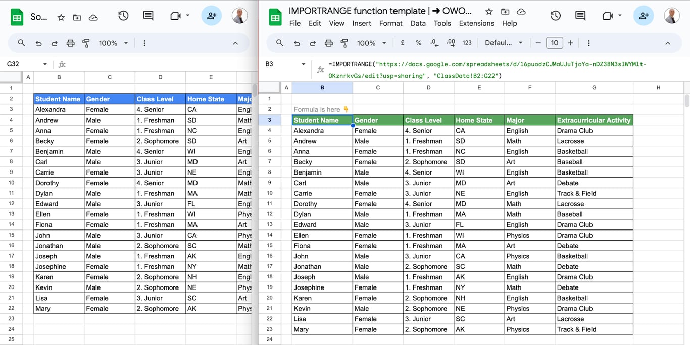
3. The cell shows #REF!. Click it and choose Allow access.
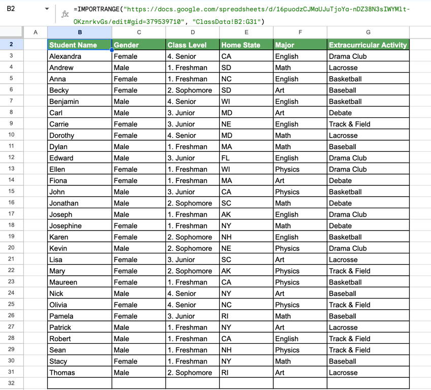
The data appears, starting in the cell with the formula. The area below and to the right of it has to be empty.
Permission is asked once for each pair of files. After that, any editor of the destination file can import any range of the source, not only the one in your formula. Keep that in mind before you connect a file that holds data some editors should not see.
OWOX Data Marts
See your first report built in real time. 15 minutes.
- Connect your data warehouse
- Pick your metrics
- Get a live Google Sheets report
In the time it takes to write a ticket. Then imagine never writing that ticket again.
Book a DemoWe'll use your actual use case
Examples of IMPORTRANGE
One tab of another file
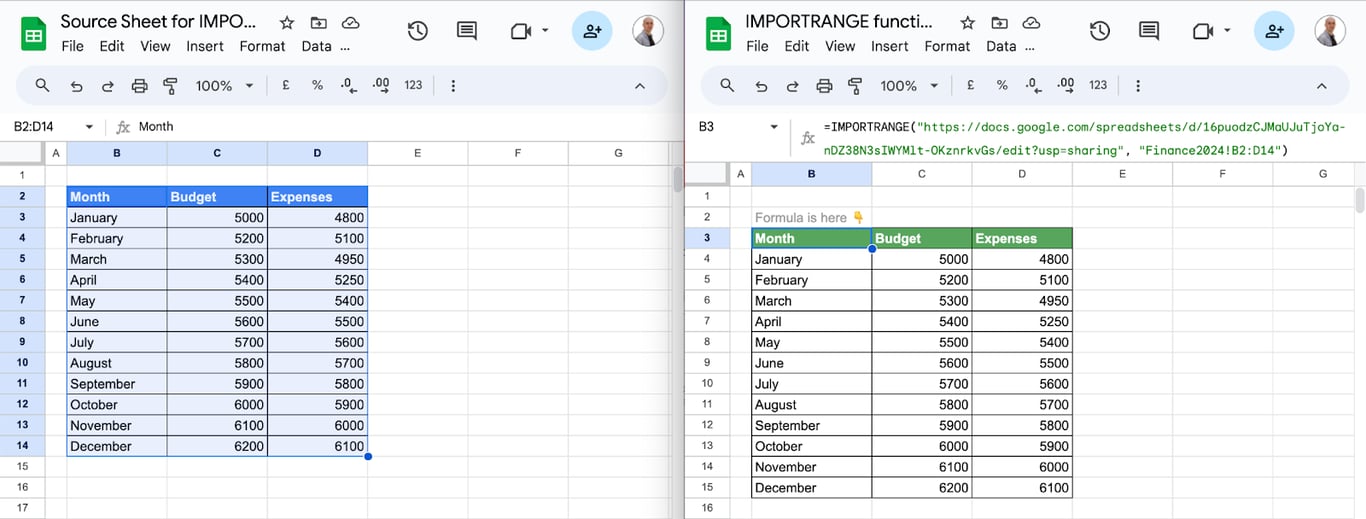
The source file has a tab for finance and a tab for sales:
=IMPORTRANGE("https://docs.google.com/spreadsheets/d/16puodzCJMaUJuTjoYa-nDZ38N3sIWYMlt-OKznrkvGs/edit", "Finance2024!B2:D14")
=IMPORTRANGE("https://docs.google.com/spreadsheets/d/16puodzCJMaUJuTjoYa-nDZ38N3sIWYMlt-OKznrkvGs/edit", "Sales2024!C2:D14")
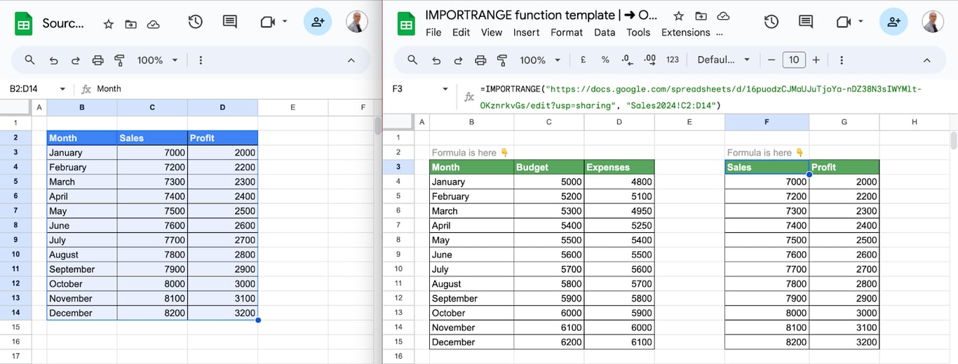
Each formula imports one range. Put them in different places of the destination file, or on different tabs.
Part of a table
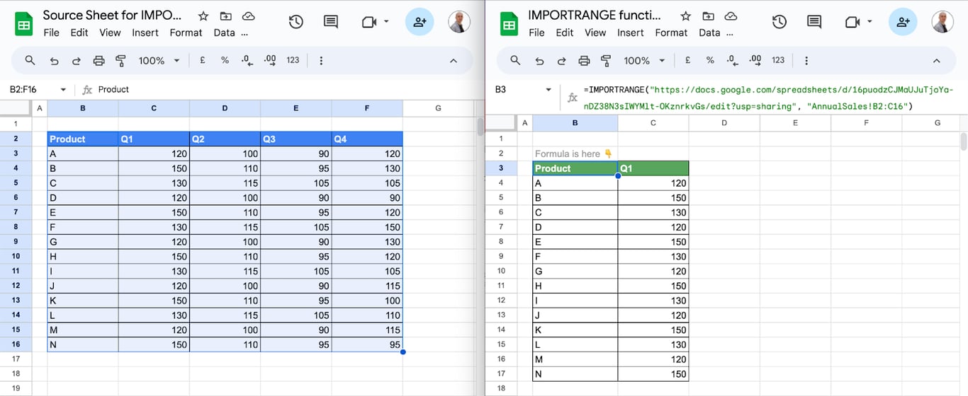
The range decides what is imported, so narrow it to the columns and rows you need. To take only the first two columns of the annual sales tab:
=IMPORTRANGE("https://docs.google.com/spreadsheets/d/16puodzCJMaUJuTjoYa-nDZ38N3sIWYMlt-OKznrkvGs/edit", "AnnualSales!B2:C16")
Several ranges in one formula
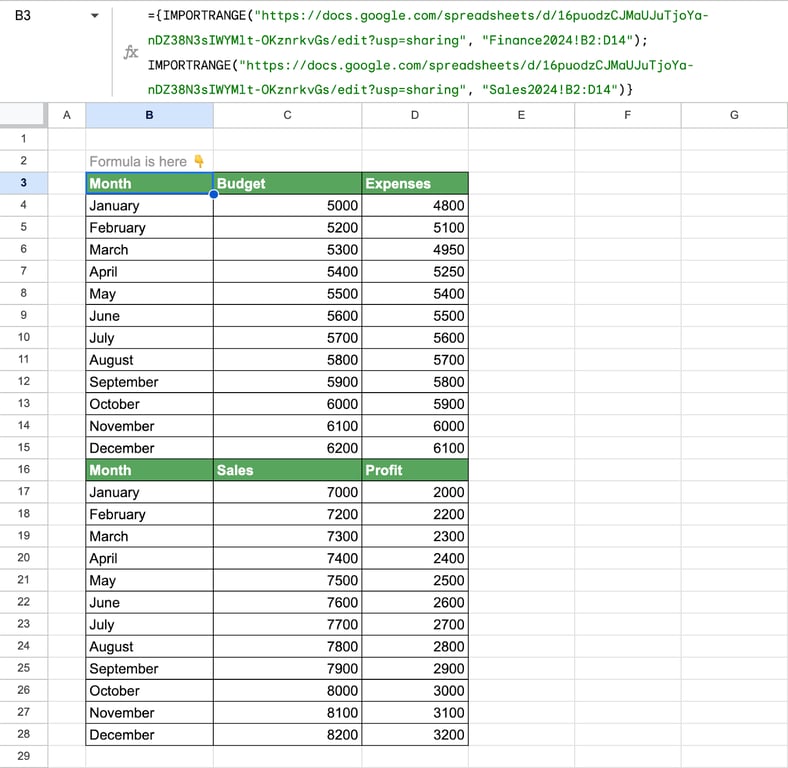
One IMPORTRANGE imports one range. To combine several, put the functions into curly braces. A semicolon stacks the results under each other:
={IMPORTRANGE("https://docs.google.com/spreadsheets/d/16puodzCJMaUJuTjoYa-nDZ38N3sIWYMlt-OKznrkvGs/edit", "Finance2024!B2:D14");
  IMPORTRANGE("https://docs.google.com/spreadsheets/d/16puodzCJMaUJuTjoYa-nDZ38N3sIWYMlt-OKznrkvGs/edit", "Sales2024!B2:D14")}
Both ranges start at their header row, so the header appears a second time in the middle of the result. Start the second range one row lower, at B3, to avoid that: in our test the two ranges then stacked into 25 rows, one header and twice twelve months.
A comma puts them side by side. (In spreadsheets set to a locale with a decimal comma, the separators inside curly braces differ.)
={IMPORTRANGE("https://docs.google.com/spreadsheets/d/16puodzCJMaUJuTjoYa-nDZ38N3sIWYMlt-OKznrkvGs/edit", "Finance2024!B2:D14"),
  IMPORTRANGE("https://docs.google.com/spreadsheets/d/16puodzCJMaUJuTjoYa-nDZ38N3sIWYMlt-OKznrkvGs/edit", "Sales2024!B2:D14")}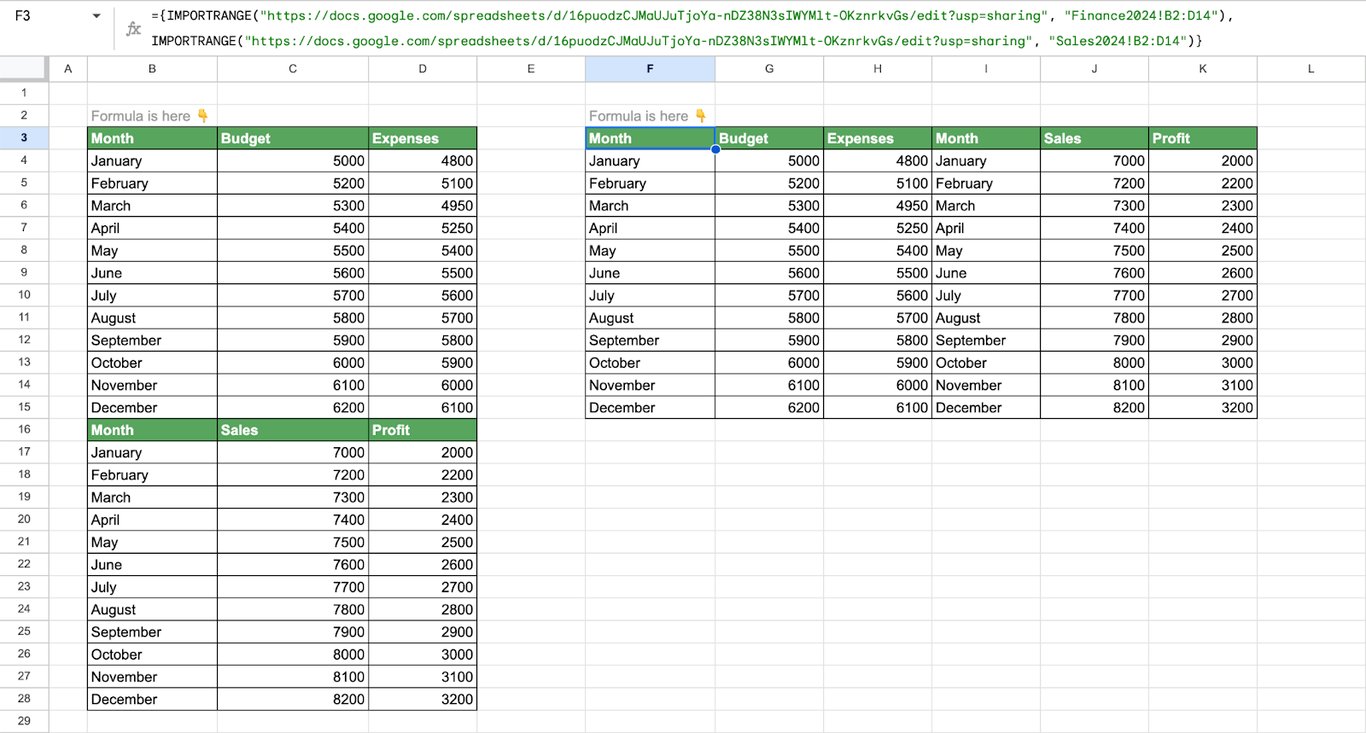
Ranges stacked with a semicolon need the same number of columns, and ranges joined with a comma need the same number of rows. Otherwise the formula returns an error. The same works for ranges from different files: use a different URL in each function, and allow access for each source.
Keep two files in sync
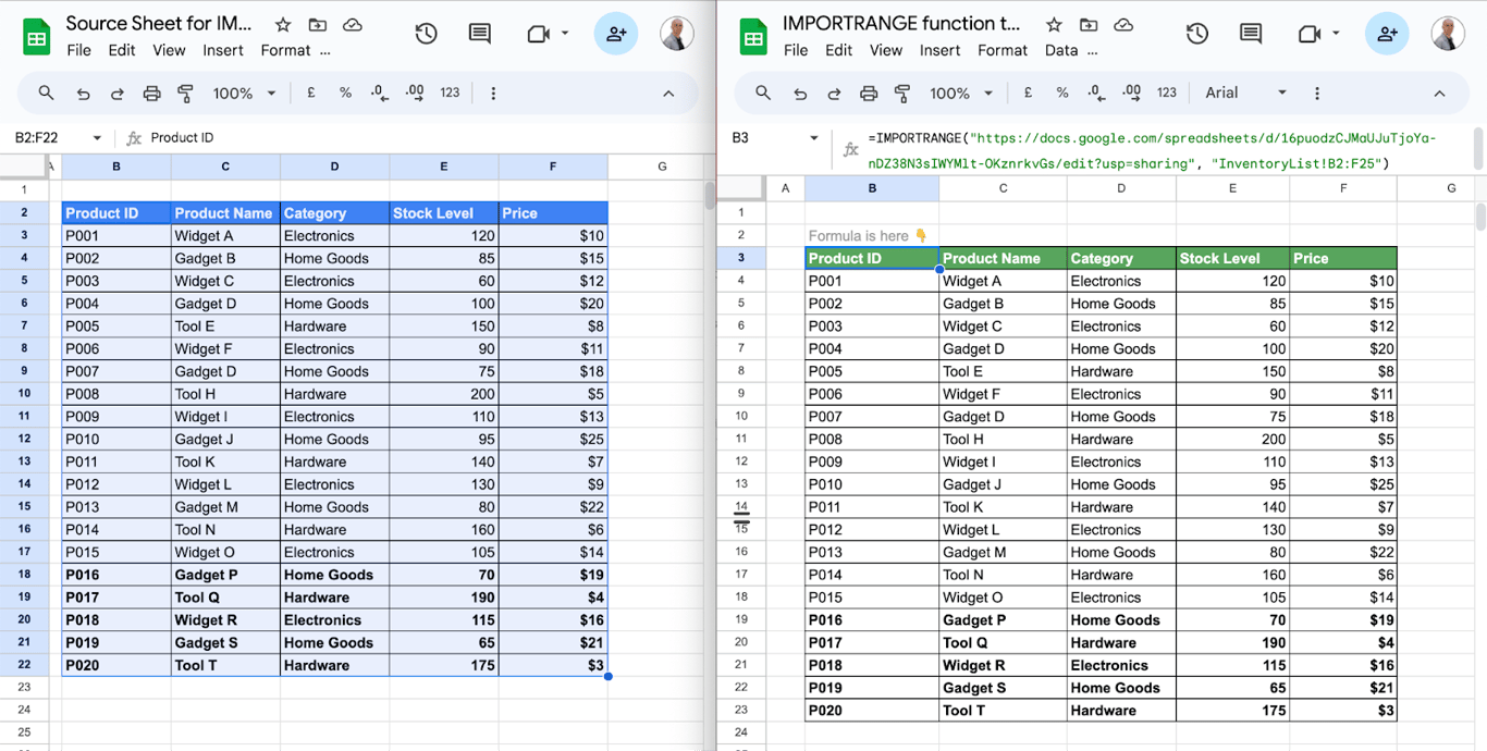
An imported range is a live link. When the source changes, the destination follows:
=IMPORTRANGE("https://docs.google.com/spreadsheets/d/16puodzCJMaUJuTjoYa-nDZ38N3sIWYMlt-OKznrkvGs/edit", "InventoryList!B2:F50")
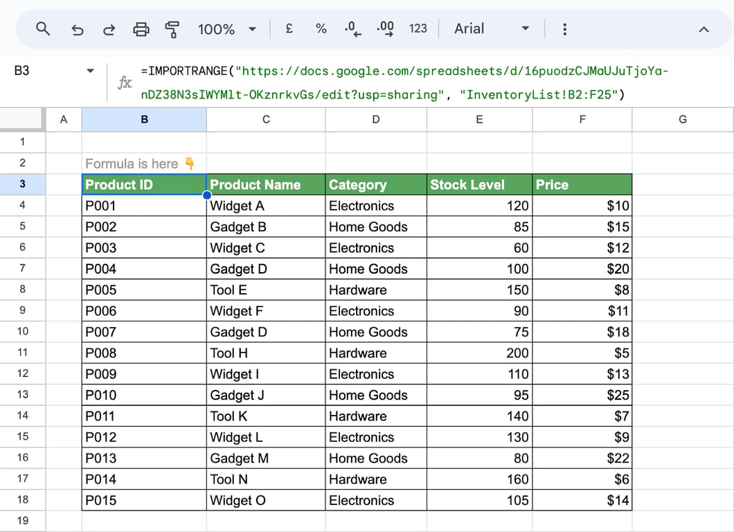
The range B2:F50 is larger than the list on purpose. When new products are added to the source, they appear in the destination without a change to the formula.
How often IMPORTRANGE refreshes
How often IMPORTRANGE refreshes
According to Google’s documentation (checked in October 2026):
- A change in the source makes every open destination file refresh. There is a delay between the change and the update.
- While the destination file is open, IMPORTRANGE also checks for updates every hour. Google’s calculation settings page gives 30 minutes for the same function; plan on up to an hour.
- Chains slow things down. If file B imports from file A and file C imports from file B, a change in A has to travel through both links.
A change usually reaches one open destination file after a short delay, and takes noticeably longer through a chain.
IMPORTRANGE with other functions
IMPORTRANGE with other functions
QUERY: filter and reorder imported data
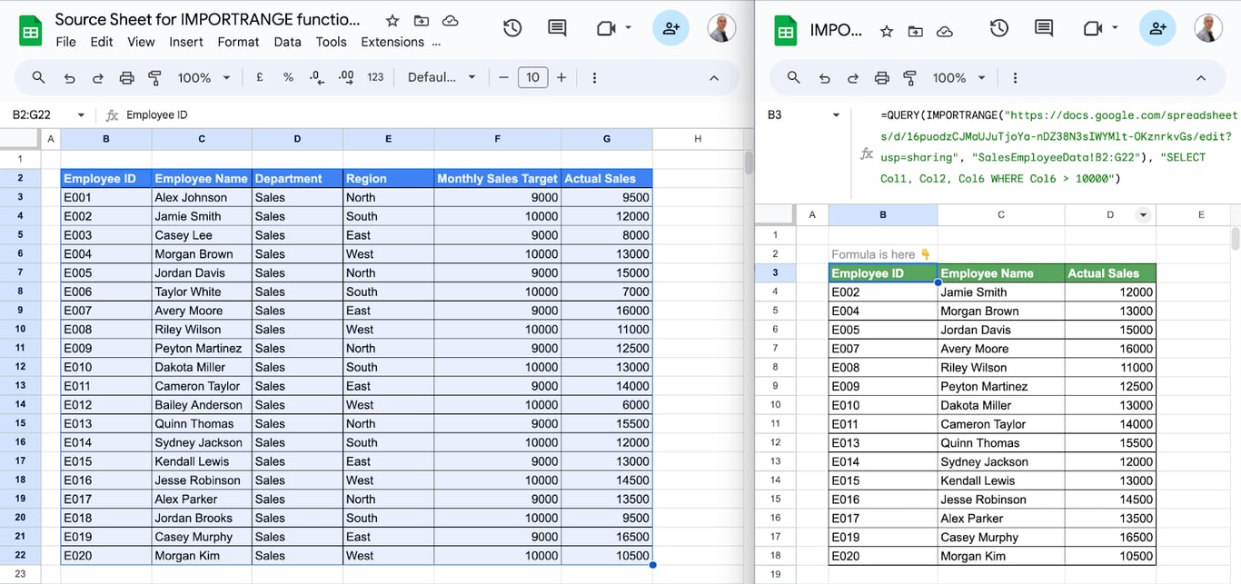
QUERY can take the imported range as its data. Because the data does not come from the sheet, columns are called Col1, Col2 and so on, counted from the first column of the imported range. To return ID, name and actual sales for employees who sold more than 10,000:
=QUERY(IMPORTRANGE("https://docs.google.com/spreadsheets/d/16puodzCJMaUJuTjoYa-nDZ38N3sIWYMlt-OKznrkvGs/edit", "SalesEmployeeData!B2:G22"), "SELECT Col1, Col2, Col6 WHERE Col6 > 10000")
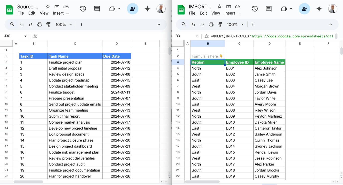
The select clause also sets the column order. This formula returns the region first, then the ID and the name:
=QUERY(IMPORTRANGE("https://docs.google.com/spreadsheets/d/16puodzCJMaUJuTjoYa-nDZ38N3sIWYMlt-OKznrkvGs/edit", "SalesEmployeeData!B2:G22"), "select Col4, Col1, Col2")
A date condition needs the date written as date 'yyyy-mm-dd'. To return the tasks that are due on or before a date seven days from today, overdue ones included:
=QUERY(IMPORTRANGE("https://docs.google.com/spreadsheets/d/16puodzCJMaUJuTjoYa-nDZ38N3sIWYMlt-OKznrkvGs/edit", "TaskList!B2:D22"), "select Col2, Col3 where Col3 <= date '" & TEXT(TODAY()+7, "yyyy-mm-dd") & "'", 1)
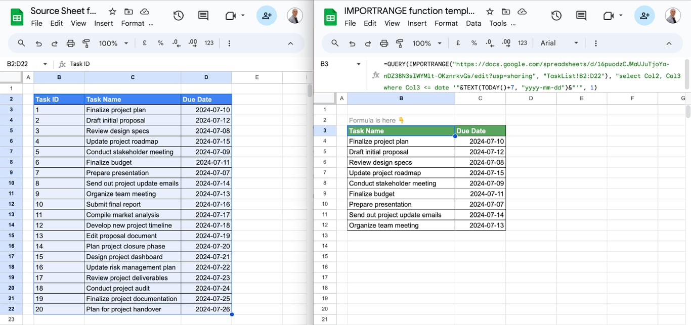
The sample tab holds dates from July 2024, so today the formula returns all twenty tasks. For a real window, add a lower bound: where Col3 >= date '2024-07-08' and Col3 <= date '2024-07-15' returned eight tasks in our test.
More on this pattern in the guides to QUERY with IMPORTRANGE and date filtering with QUERY.
VLOOKUP: look up a value in another file
Use the imported range as the table of VLOOKUP:
=VLOOKUP(B3, IMPORTRANGE("https://docs.google.com/spreadsheets/d/16puodzCJMaUJuTjoYa-nDZ38N3sIWYMlt-OKznrkvGs/edit", "SalesEmployeeData!B2:G22"), 2, FALSE)
- B3: the employee ID to look for.
- IMPORTRANGE(…): the employee table in the other file, with the IDs in its first column.
- 2: the second column of that range, the name.
- FALSE: exact match.
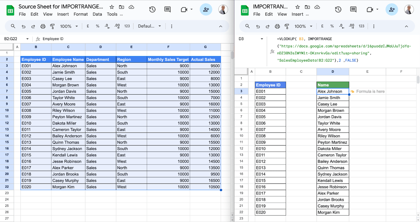
Copied down a long column, this formula asks for the same range in every row. It is faster to import the table once to a helper tab and point the lookups at that tab.
FILTER: rows that meet a condition
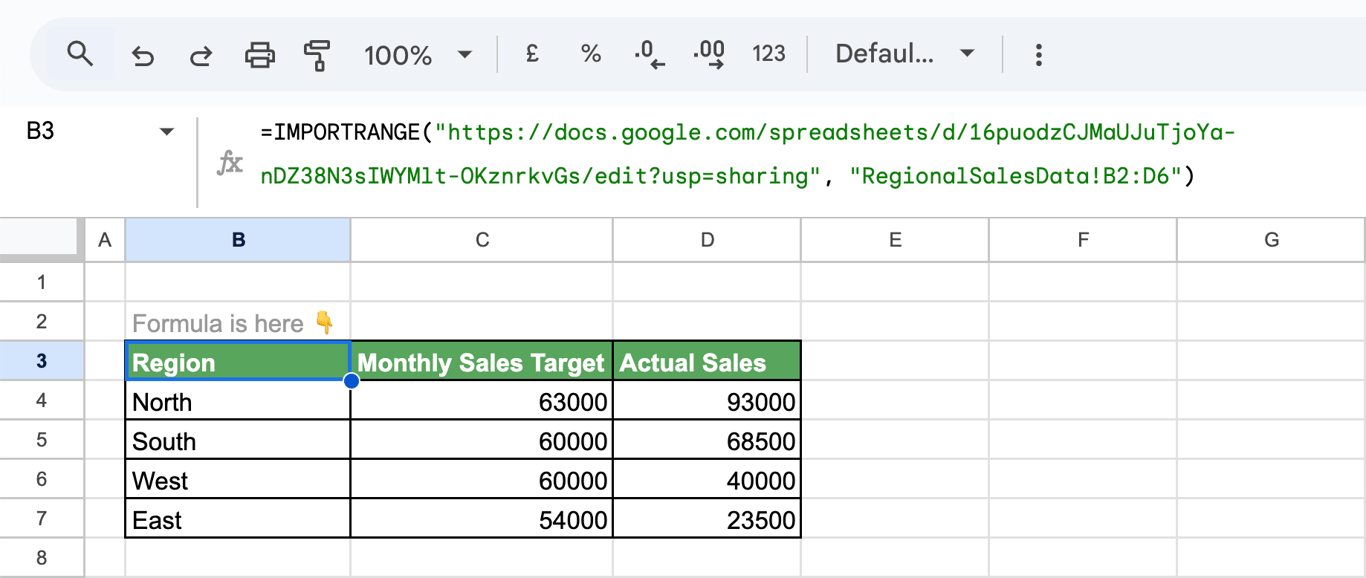
Import the range first, then filter the imported cells. In the screenshots the import formula sits in B3, so the header lands in row 3 and the data in B4:D7:
=IMPORTRANGE("https://docs.google.com/spreadsheets/d/16puodzCJMaUJuTjoYa-nDZ38N3sIWYMlt-OKznrkvGs/edit", "RegionalSalesData!B2:D6")
=FILTER(B4:D7, D4:D7 > C4:C7)
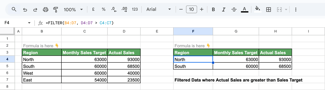
FILTER returns the regions where the actual sales are higher than the target: North and South in the sample data. The same in one formula, with QUERY: =QUERY(IMPORTRANGE("url", "RegionalSalesData!B2:D6"), "select * where Col3 > Col2", 1).
SUM: a total across files
Aggregate functions accept the imported range directly. To add up the expenses of two departments kept on two tabs:
=SUM(IMPORTRANGE("https://docs.google.com/spreadsheets/d/16puodzCJMaUJuTjoYa-nDZ38N3sIWYMlt-OKznrkvGs/edit", "DeptA Expenses!C3:C22"), IMPORTRANGE("https://docs.google.com/spreadsheets/d/16puodzCJMaUJuTjoYa-nDZ38N3sIWYMlt-OKznrkvGs/edit", "DeptB Expenses!C3:C22"))
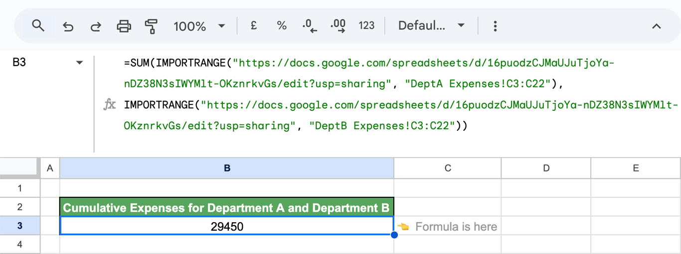
SUMIF and COUNTIF are different: they need a real range in the sheet and do not accept the result of IMPORTRANGE. Use QUERY with a where clause, or import the data to a tab first. When the total is all you need, Google’s advice is to calculate it in the source file and import the single cell: less data travels between the files.
Limits of IMPORTRANGE
The same documentation lists the first four of these limits; the fifth is how the function behaves:
- 10 MB per request. A range that returns more data fails with #ERROR! and “Result too large”.
- Too many import requests are throttled. The cell shows “Loading…” with a note that loading may take a while. The quota belongs to the creator of the file and covers all import functions in all their open files.
- No volatile functions. IMPORTRANGE cannot refer, directly or through other cells, to a cell with NOW, RAND or RANDBETWEEN. TODAY is allowed.
- Access counts as a share. Each connected destination file counts toward the limit of 600 users a source file can be shared with.
- Values only. Formatting, formulas, comments and validation rules of the source are not imported.
For large tables and scheduled loads, Google itself points to other tools in that article, among them Connected Sheets.
IMPORTRANGE errors
#REF!: you need to connect these sheets
⚠️ Error: #REF! with a prompt to allow access.
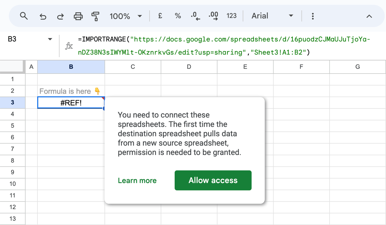
✅ Solution: Click the cell and choose Allow access. If there is no button, you do not have access to the source file: open its URL in the browser and request access from the owner.
#REF!: cannot find range or sheet
⚠️ Error: #REF! with “Cannot find range or sheet for imported range”.
=IMPORTRANGE("https://docs.google.com/spreadsheets/d/16puodzCJMaUJuTjoYa-nDZ38N3sIWYMlt-OKznrkvGs/edit", "Sheet3!A1:B2")
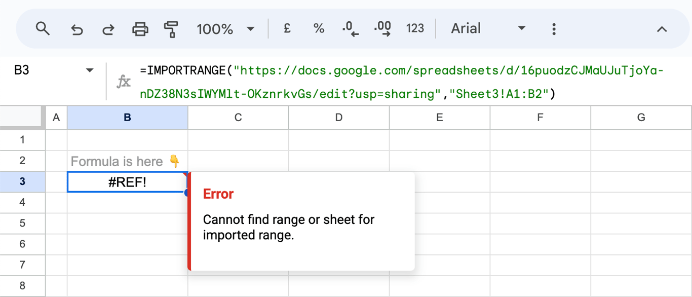
✅ Solution: The tab name or the range in the second argument does not exist in the source. Copy the tab name exactly, including spaces. Capitals do not matter: in our test “regionalsalesdata” found the tab RegionalSalesData.
#REF!: the result has no room
⚠️ Error: #REF! with “Array result was not expanded because it would overwrite data”.
✅ Solution: Something is already in the cells where the import should land. Clear them or move the formula.
#ERROR!: formula parse error
⚠️ Error: #ERROR! right after typing or pasting the formula.
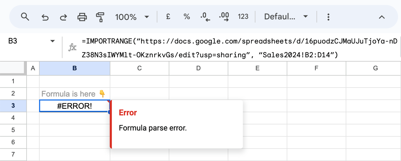
✅ Solution: Most often the quotation marks are typographic ones (“ ”), which arrive with a formula copied from a document or a web page. Retype them as straight quotes. Also check the comma between the two arguments and the closing parenthesis.
#ERROR!: result too large
⚠️ Error: #ERROR! with “Result too large”.
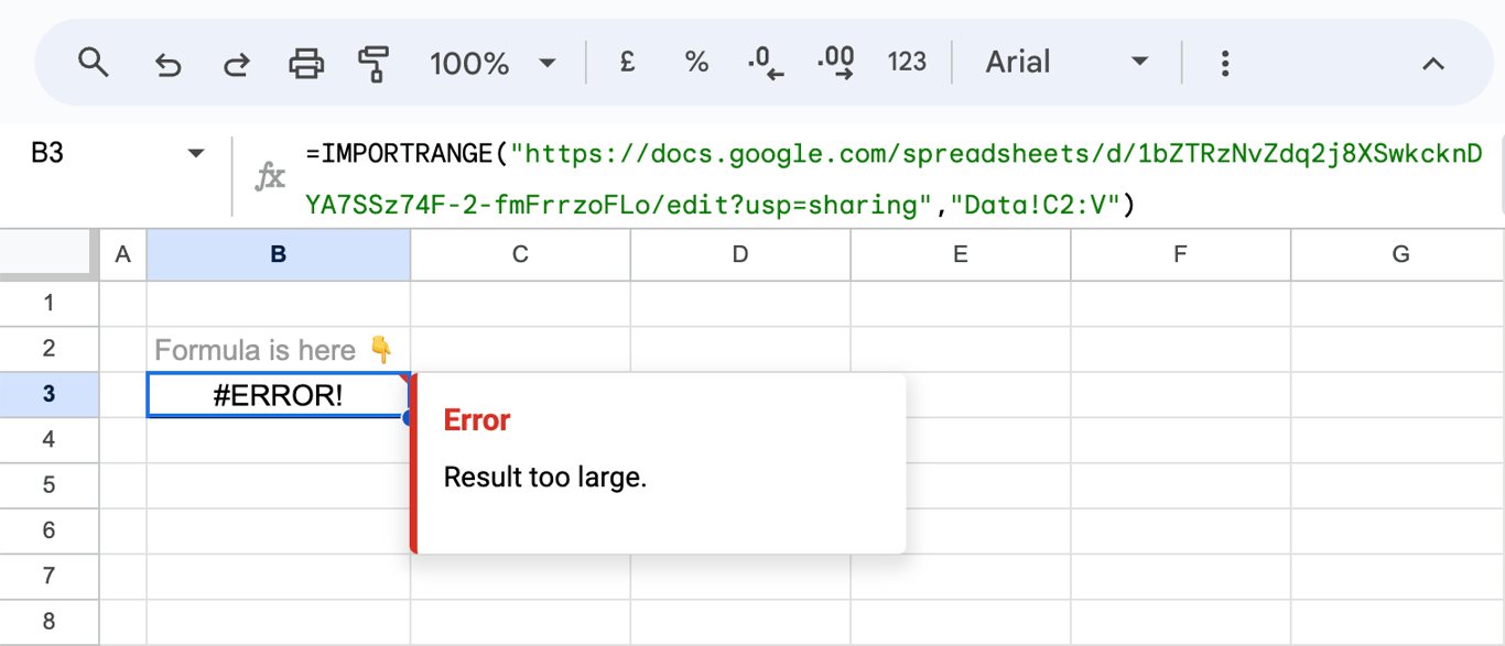
✅ Solution: The range returns more than 10 MB. Import fewer columns or rows, split the range into several formulas, or summarize the data in the source file and import the summary.
The data stopped updating
⚠️ Error: The destination shows old values or stays on “Loading…”.
✅ Solution: Check that the person who allowed access still has access to the source: the link lasts only as long as that person does. Then cut the formula out of the cell and paste it back, which makes IMPORTRANGE load again. Reloading the page is not a reliable way to force it.
Related Google Sheets functions
Related Google Sheets functions
Functions that are often used next to IMPORTRANGE, each with its own guide:
- QUERY with IMPORTRANGE: Filtering and aggregating imported data in detail.
- Linking data across sheets: References between tabs and files.
- IMPORTDATA: Imports a CSV or TSV file from a URL.
- IMPORTXML, IMPORTHTML and IMPORTFEED: Import data from web pages and feeds.
- FILTER: Returns the rows that meet a condition.
- XLOOKUP: A lookup that searches in any direction.
- UNIQUE: Returns the distinct values of a range.
- Pivot tables: Summarize the imported table by category.
IMPORTRANGE links spreadsheets; the data still has to get into one of them
IMPORTRANGE links spreadsheets; the data still has to get into one of them
IMPORTRANGE moves data between Google Sheets files. It does not solve the step before that: getting the orders, the ad spend or the CRM records into a spreadsheet at all. If the data in the source file was itself exported and pasted in, IMPORTRANGE only passes that copy on.
The OWOX Data Marts extension for Google Sheets covers that half. A data analyst publishes a data mart (a table or an SQL query in your data warehouse) and makes it available for reports. In Sheets you open the extension, pick the data mart, tick the columns you want and run it. The rows land in a tab, ready for your formulas.
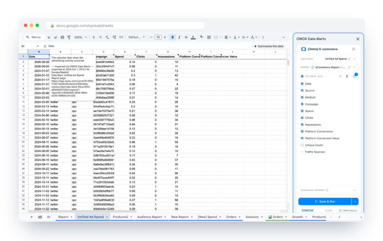
What changes for the person who maintains the sheet:
- Refresh replaces re-export. Refresh current report in the extension menu re-runs the same pull, and a scheduled refresh keeps the tab current without anyone touching it. Which cells that refresh rewrites, and where your own formulas are safe, is in our guide to refreshes and formulas.
- The source is written on the sheet. The header cell of an imported tab carries a note with the data mart it came from, the time of the import and a link to the report.
- No SQL and no warehouse access needed. The analyst decides which data marts and columns are available. You choose from that list.
The extension does not write or change the analyst’s SQL. Each report reads the data mart it needs directly, so there is no master spreadsheet to keep alive and no chain of imports behind the numbers. The extension comes with the OWOX Cloud plans of OWOX Data Marts; spreadsheet reporting describes both ways data reaches a sheet.
Turn your data into decisions.
Governed data marts give you the clean foundation ML needs to actually work.
- No AI hallucinations
- Analyst-governed definitions
- Every number traces to SQL
Frequently Asked Questions
Can you use IMPORTRANGE in the same sheet?
IMPORTRANGE is meant for another spreadsheet file. For a range on another tab of the same file, a plain reference such as =Sheet2!A1:C10, or ={Sheet2!A1:C10} for the whole range, is simpler, needs no permission and updates instantly.
Can IMPORTRANGE include formatting?
No. IMPORTRANGE imports values only. Number formats, colours, conditional formatting, data validation rules and the formulas behind the values stay in the source file; format the imported range in the destination file.
What are the limitations of IMPORTRANGE?
Google documents several: one request returns at most 10 MB of data; too many import requests are throttled and show Loading; the function cannot refer to cells with NOW, RAND or RANDBETWEEN; each connected file counts toward the 600-user sharing limit of the source; and only values are imported, without formatting. Updates arrive with a delay, and the function checks for changes every hour while the file is open.
What is the difference between IMPORTRANGE and query in Google Sheets?
IMPORTRANGE imports data from another Google Sheet, while query allows you to perform SQL-like queries within your sheet to manipulate and filter your data. Query works on data already in your sheet or imported via IMPORTRANGE, providing more control over data analysis.
How does IMPORTRANGE work in Google Sheets?
IMPORTRANGE lets you import data from one Google Sheet into another. By specifying the source sheet's URL and the range of cells you want to import, you can seamlessly integrate data across multiple sheets, facilitating centralized data management and analysis.
What is the difference between IMPORTRANGE and IMPORTDATA in Google Sheets?
IMPORTRANGE allows you to bring data from one Google Sheet into another, while IMPORTDATA is used to import data from a web URL, typically in CSV or TSV format. IMPORTRANGE is for sheet-to-sheet data transfer, and IMPORTDATA fetches data from the web.