FILTER function in Google Sheets: formula, conditions and examples
FILTER returns the rows of a range that meet one or more conditions and updates when the data changes. This guide covers the formula, AND and OR conditions, filtering by text, number, date and time, FILTER combined with SORT, UNIQUE, SUM and LARGE, and the errors the function returns.

The FILTER function returns the rows of a range that meet a condition:
=FILTER(B3:E17, B3:B17 = "John Doe")
The result is a live copy of the matching rows. It is recalculated whenever the source data changes, and the source itself stays as it is, which is the difference from the filter in the Data menu.
| You need | Formula |
|---|---|
| One condition | =FILTER(B3:E17, C3:C17 = "Financial Software") |
| Two conditions, both true (AND) | =FILTER(B3:E17, C3:C17 = "Financial Software", E3:E17 > 5000) |
| Either of two conditions (OR) | =FILTER(B3:E17, (C3:C17 = "Financial Software") + (C3:C17 = "Marketing Analytics")) |
| Everything except a value | =FILTER(B3:E17, B3:B17 <> "John Doe") |
| Text that contains a word | =FILTER(B3:E17, REGEXMATCH(C3:C17, "Software")) |
| Rows after a date | =FILTER(B3:E17, D3:D17 > DATE(2023,1,17)) |
| A message when nothing matches | =IFERROR(FILTER(B3:E17, B3:B17 = "Angela Davis"), "No matching data found") |
FILTER syntax
=FILTER(range, condition1, [condition2, ...])
- range: the data to filter. It can have one column or many.
- condition1: a column (or row) of TRUE and FALSE values, usually a comparison such as B3:B17 = “John Doe”. It must have the same number of rows as the range.
- condition2, … (optional): more conditions. A row is returned only when all of them are TRUE.
Type the formula into the cell where the result should start. The rows fill the cells below and to the right of it, so that area has to be empty.
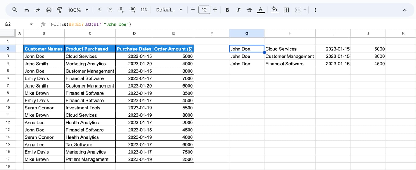
The formula returns the three orders made by John Doe. To filter data that sits on another tab, add the tab name to each range: =FILTER(Sheet1!A2:B10, Sheet1!A2:A10 = "criteria").
Filter by one condition
Text
To return the rows where the product is “Financial Software”:
=FILTER(B3:E17, C3:C17 = "Financial Software")
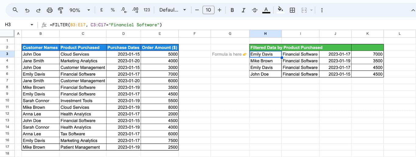
The comparison looks for the whole cell value. For cells that contain a word, use REGEXMATCH inside the condition: =FILTER(B3:E17, REGEXMATCH(C3:C17, "Software")) returns every product with “Software” in its name. The guide to REGEX functions explains the patterns.
Numbers
=FILTER(B3:E17, E3:E17 > 6000)
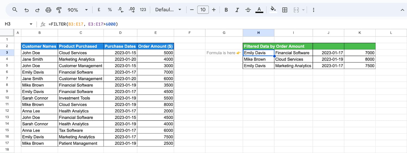
The formula returns the orders above $6,000. All comparison operators work: >, <, >=, <=, = and <>.
Dates
Write the date with the DATE function, so that it is read the same way in every locale:
=FILTER(B3:E17, D3:D17 > DATE(2023,1,17))
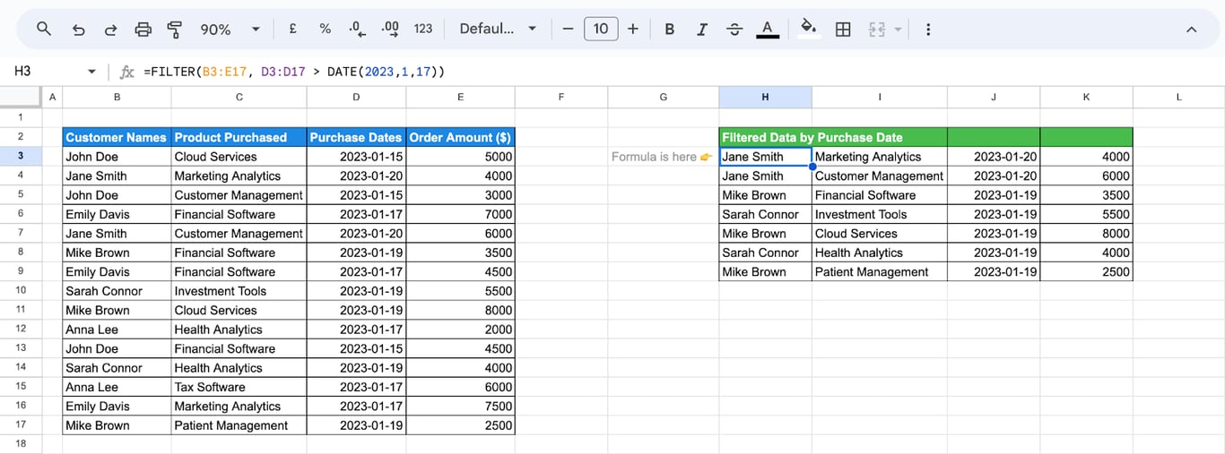
The formula returns the purchases made after January 17, 2023. For a period, add a second condition: =FILTER(B3:E17, D3:D17 >= DATE(2023,1,17), D3:D17 <= DATE(2023,1,19)).
Time
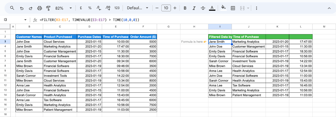
With a column for the time of purchase, compare it with a value built by TIME:
=FILTER(B3:E17, TIMEVALUE(E3:E17) > TIME(10,0,0))
- B3:E17: the range, here with the time of purchase in column E.
- TIMEVALUE(E3:E17): the time of each row as a time value. It is needed when the times are stored as text; with real time values,
E3:E17 > TIME(10,0,0)is enough. - TIME(10,0,0): 10:00 AM.
OWOX Data Marts
See your first report built in real time. 15 minutes.
- Connect your data warehouse
- Pick your metrics
- Get a live Google Sheets report
In the time it takes to write a ticket. Then imagine never writing that ticket again.
Book a DemoWe'll use your actual use case
Filter by several conditions
AND: all conditions true
Conditions listed one after another, separated by commas, all have to be true. The same can be written as a multiplication of the conditions, each in its own parentheses:
=FILTER(B3:E17, (C3:C17 = "Financial Software") * (E3:E17 > 5000))
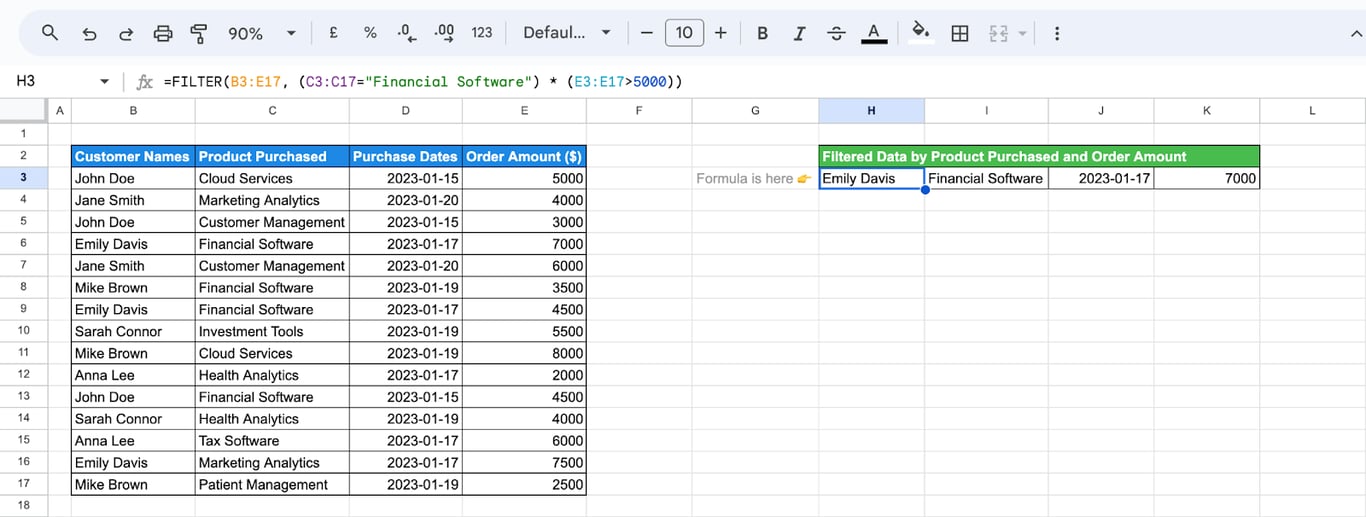
TRUE counts as 1 and FALSE as 0, so the product is 1 only when both conditions hold. The result here is one row: Financial Software with an order amount above $5,000.
OR: at least one condition true
For OR, add the conditions instead of multiplying them:
=FILTER(B3:E17, (C3:C17 = "Financial Software") + (C3:C17 = "Marketing Analytics"))
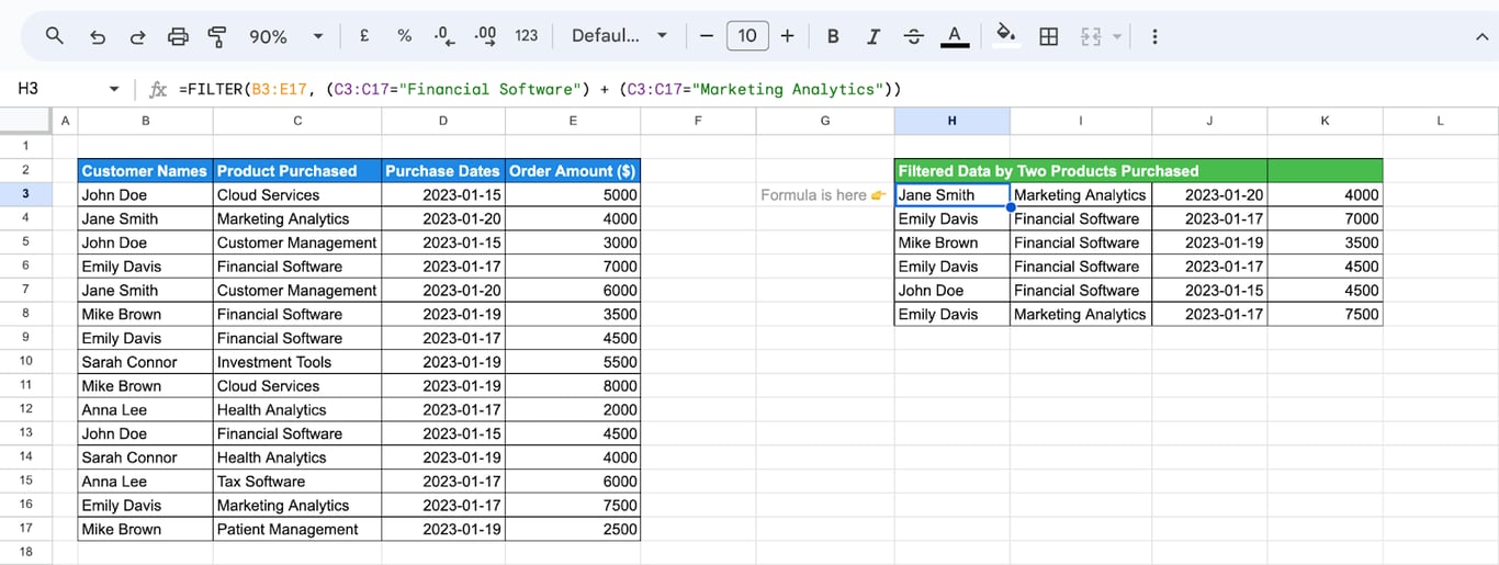
A row is returned when the sum is 1 or more, that is, when at least one condition is true. The functions AND and OR cannot be used here: they reduce the whole column to a single TRUE or FALSE.
FILTER with other functions
SORT: put the result in order
Wrap FILTER in SORT to order the rows it returns:
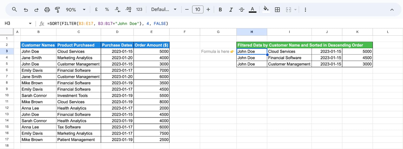
=SORT(FILTER(B3:E17, B3:B17 = "John Doe"), 4, FALSE)
- FILTER(B3:E17, B3:B17 = “John Doe”): the orders of John Doe.
- 4: sort by the fourth column of the result, the order amount.
- FALSE: descending order, largest first.
UNIQUE: remove duplicates
=UNIQUE(FILTER(B3:B17, B3:B17 <> ""))
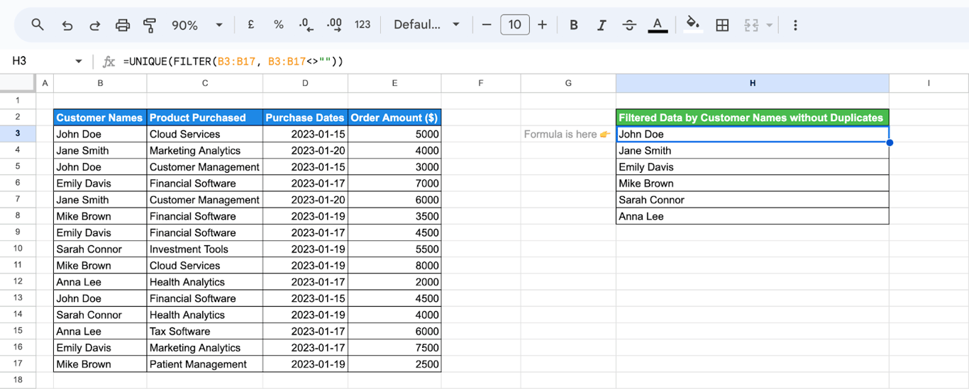
FILTER drops the empty cells and UNIQUE returns each customer name once.
SUM: add up the matching rows
=SUM(FILTER(E3:E17, B3:B17 = "John Doe"))
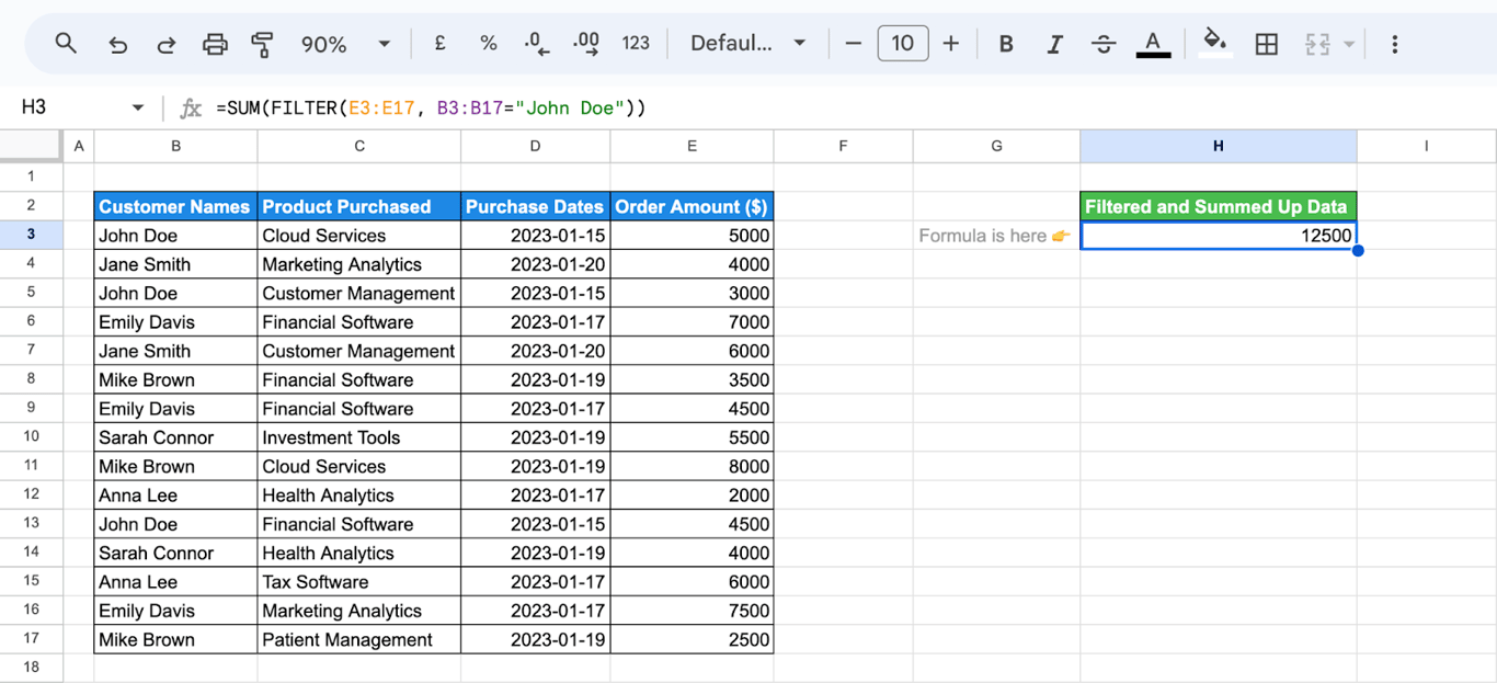
FILTER returns the order amounts of John Doe and SUM adds them: 12,500. For a simple condition like this one, =SUMIF(B3:B17, "John Doe", E3:E17) gives the same total; FILTER is worth using when the condition is one that SUMIF cannot express, such as an OR across two columns.
LARGE: the largest value among the matching rows
=LARGE(FILTER(E3:E17, B3:B17 = "John Doe"), 1)
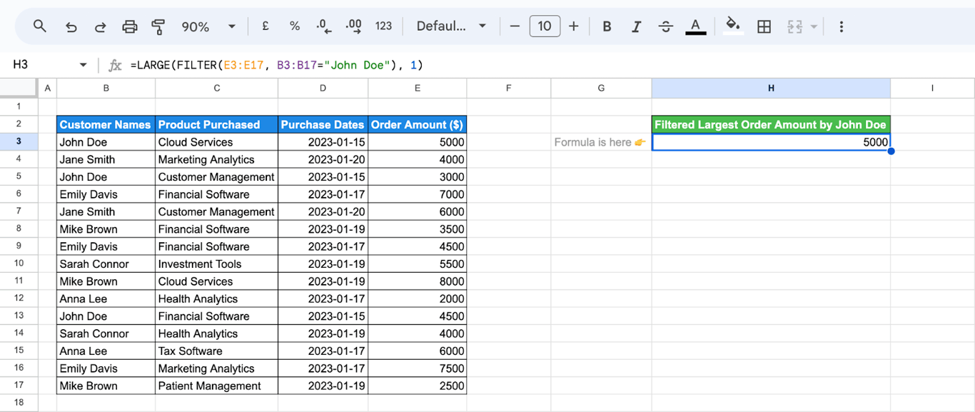
The 1 asks for the largest value; 2 would return the second largest.
The top 3 rows
LARGE can also sit inside the condition. This formula returns the rows whose amount is at least as large as the third largest amount:
=FILTER(B3:E17, E3:E17 >= LARGE(E3:E17, 3))
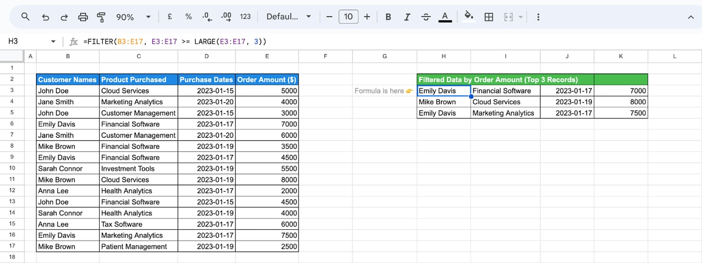
When two rows tie for third place, both are returned, and the result has four rows. For exactly three, sort and cut: =SORTN(SORT(B3:E17, 4, FALSE), 3).
FILTER errors
Mismatched range sizes
⚠️ Error: #N/A with “FILTER has mismatched range sizes”.
=FILTER(B3:C17, A3:A15 = "John Doe", A3:A15 = "Emily Davis")
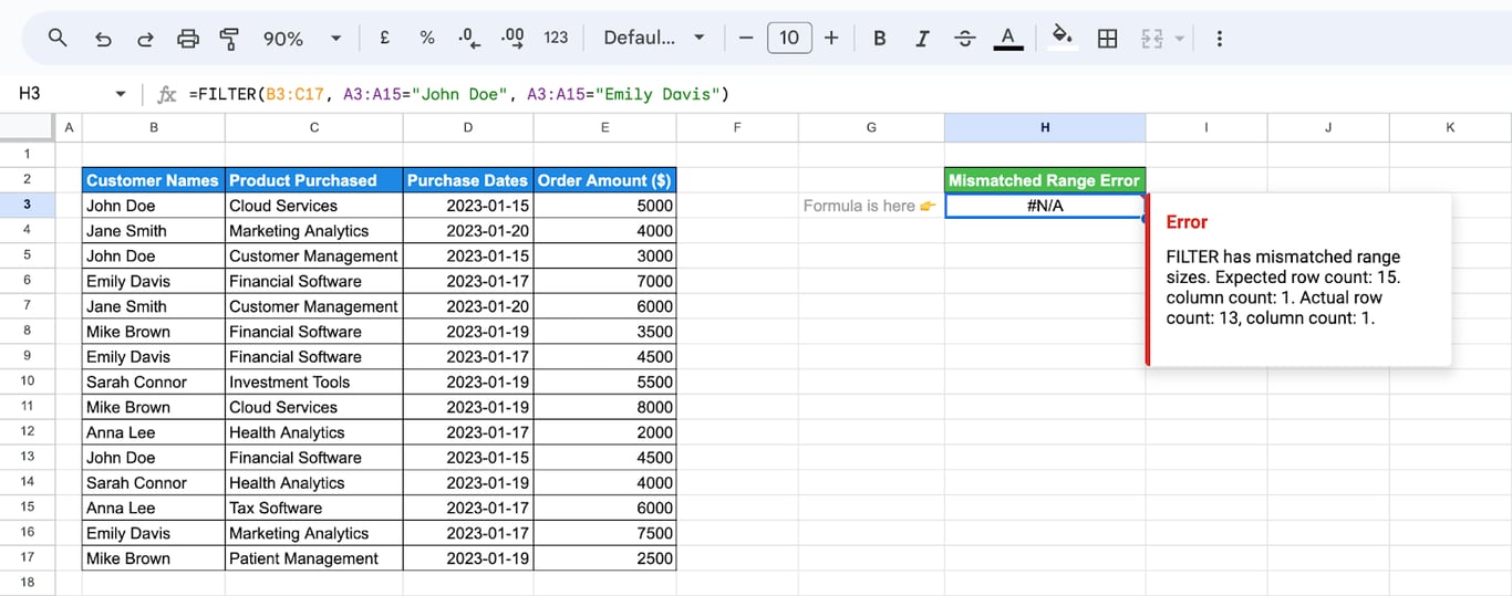
✅ Solution: The range has 15 rows (3 to 17) and the conditions have 13 (3 to 15). Make every condition cover the same rows as the range. This formula has a second problem: two conditions separated by a comma both have to be true, and a name cannot be “John Doe” and “Emily Davis” at once. For either name, add the conditions with +.
#REF!: no room for the result
⚠️ Error: #REF! with “Array result was not expanded because it would overwrite data”.
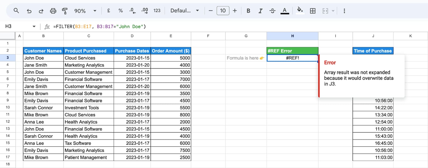
✅ Solution: A cell in the area where the result should appear already has content. Clear it, or move the formula to a place with enough empty cells below and to the right.
#N/A: no matches
⚠️ Error: #N/A with “No matches are found in FILTER evaluation”.
=FILTER(B3:E17, B3:B17 = "Angela Davis")
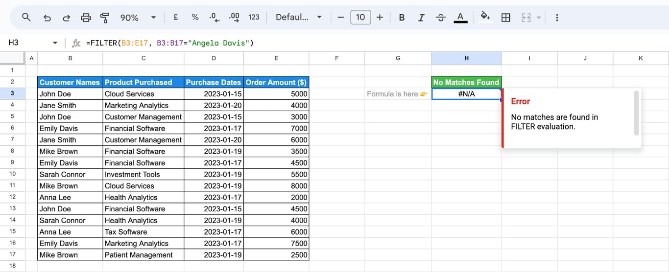
✅ Solution: No row meets the condition. To show a message instead of the error, wrap the formula in IFERROR:
=IFERROR(FILTER(B3:E17, B3:B17 = "Angela Davis"), "No matching data found")
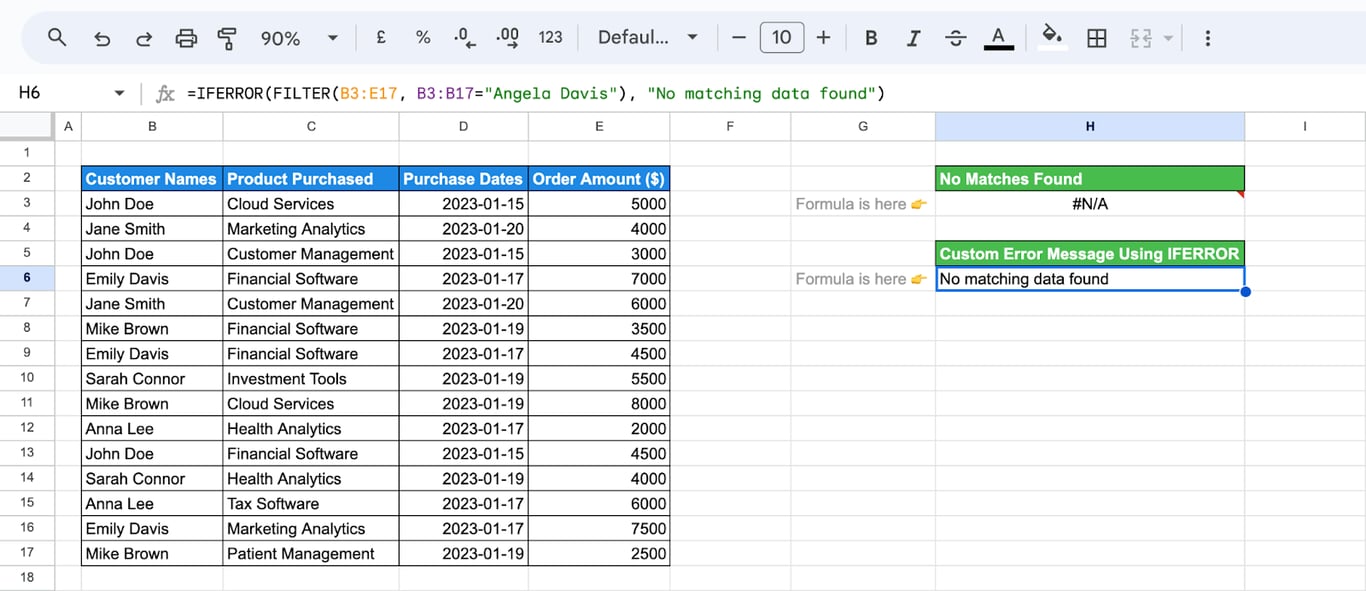
Keep this error in mind when FILTER is inside a counting function: =COUNTA(FILTER(...)) returns 1 when nothing matches, because the error itself is counted.
The result cannot be edited
⚠️ Error: Typing into a cell of the result breaks the formula.
✅ Solution: Only the first cell holds the formula; the others are its output. To change the result, change the conditions or the source data. To get an editable copy, copy the result and paste it elsewhere with Edit > Paste special > Values only.
Related Google Sheets functions
Related Google Sheets functions
Functions that are often used with or instead of FILTER, each with its own guide:
- QUERY: Filters, sorts and aggregates in one formula with SQL-like syntax.
- SORT and SORTN: Order a range and return the first rows of it.
- UNIQUE: Returns the distinct values of a range.
- ARRAYFORMULA: Applies a formula to a whole range.
- XLOOKUP and VLOOKUP: Return one matching row for a key, where FILTER returns all of them.
- Slicers: Adds on-sheet filter controls for pivot tables and charts.
- Exploratory data analysis: Walks through summarising and visualising a dataset before building reports on it.
- SPLIT: Divides the text in a cell into separate columns around a delimiter such as a comma or a space.
FILTER works on what is already in the tab
FILTER works on what is already in the tab
A FILTER formula narrows down rows that someone has brought into the spreadsheet. When those rows come from a full export of a CRM or an ad platform, most of the sheet is data that only exists to be filtered away, and it has to be exported again before every report.
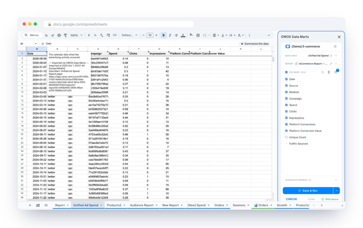
The OWOX Data Marts extension for Google Sheets covers that half. A data analyst publishes a data mart (a table or an SQL query in your data warehouse) and makes it available for reports. In Sheets you open the extension, pick the data mart, tick the columns you want and run it. The rows land in a tab, ready for your formulas.
What changes for the person who maintains the sheet:
- Refresh replaces re-export. Refresh current report in the extension menu re-runs the same pull, and a scheduled refresh keeps the tab current without anyone touching it.
- The source is written on the sheet. The header cell of an imported tab carries a note with the data mart it came from, the time of the import and a link to the report.
- No SQL and no warehouse access needed. The analyst decides which data marts and columns are available. You choose from that list.
The extension does not write or change the analyst’s SQL. The first cut, which rows and which columns the report needs at all, is made there, and FILTER handles the views on top of it. The extension comes with the OWOX Cloud plans of OWOX Data Marts; spreadsheet reporting describes both ways data reaches a sheet.
Turn your data into decisions.
Governed data marts give you the clean foundation ML needs to actually work.
- No AI hallucinations
- Analyst-governed definitions
- Every number traces to SQL
Frequently Asked Questions
Can the FILTER function apply multiple conditions to data?
Yes. Conditions separated by commas all have to be true: =FILTER(A2:C, B2:B = "East", C2:C > 100). For OR, add the conditions in parentheses: =FILTER(A2:C, (B2:B = "East") + (B2:B = "West")). The AND and OR functions do not work inside FILTER, because they return a single value for the whole column.
What are some advanced uses of the FILTER function?
Advanced uses of the FILTER function include sorting filtered data, combining FILTER with other functions like UNIQUE or SUM, and using it with array formulas for more complex analysis.
What should I do if my FILTER function is not working as expected?
Read the message in the cell. Mismatched range sizes means a condition covers different rows than the range. #REF! means the result has no room, so clear the cells below and to the right of the formula. #N/A with No matches means no row meets the conditions; wrap the formula in IFERROR to show your own text.
How can I avoid common errors while using the FILTER function?
To avoid common errors while using the FILTER function, ensure that all ranges in the formula match in size, and keep surrounding cells empty to prevent #REF! errors, and handle situations where no matches are found using IFERROR statements.
How do you start using the FILTER function on a dataset?
To start using the FILTER function, select the range of data you want to filter, then input the formula =FILTER(range, condition) where "range" is the data you want to filter, and "condition" is the criteria you want to apply.
What exactly is the FILTER function in Google Sheets?
The FILTER function in Google Sheets is a tool used to extract specific data from a dataset based on defined criteria, showing only the rows that meet those conditions.