Snowflake Pricing Explained: Compute Credits, Storage, and Cost Control

Snowflake is incredibly attractive on paper: fully managed, near-infinite scalability, pay only for what you use. In practice, many teams discover something else a few months into adoption – invoices that climb faster than planned, and no clear story of why.

If you’re a Data Analyst, Analytics Engineer, BI Developer, or analytics lead, you’ve probably felt this tension. Stakeholders love the speed and flexibility. Finance asks why the “data warehouse” line item doubled last quarter. And somewhere between those two perspectives sits your data architecture.

This guide breaks down Snowflake pricing from a practitioner’s point of view – not just what Snowflake charges for, but how your reporting and transformation patterns directly drive those charges. You’ll learn:

• How Snowflake compute credits, warehouses, and storage really work in 2026
• Why reporting and BI workflows often create unpredictable, spiky compute usage
• How to design governed Data Marts and analytic layers that keep Snowflake as your source of truth while reducing waste
• Practical levers you can pull (architecture, governance, and tooling) to keep performance high and costs under control

By the end, you should be able to look at your current Snowflake setup, tie technical choices to budget impact, and design a roadmap for sustainable cost optimization – without slowing down your analysts or starving the business of insights.

Why Snowflake Costs Feel Hard to Predict

Snowflake’s marketing emphasizes simplicity: three main dimensions of cost – compute, storage, and data transfer. From a contract perspective, this is accurate. From an operations perspective, it’s incomplete.

In real-world analytics environments, most unexpected costs don’t come from storage or obvious heavy jobs. They come from:

• Ad-hoc exploratory queries that scan large raw tables
• BI dashboards that re-compute the same aggregations dozens or hundreds of times per day
• Un-governed dbt models or scheduled jobs that overlap in time and spike warehouse concurrency
• Multiple teams spinning up their own warehouses without shared standards

All of this is powered by Snowflake’s flexible, consumption-based model. The same design that lets you run a complex model in minutes instead of hours will happily let 50 near-identical dashboards each run their own full-table scans.

The key idea for this article: your reporting architecture – not just your volume of data – is what really drives your Snowflake compute bill. We’ll keep returning to this point as we unpack each pricing component and then connect it to design choices you control.

Snowflake Compute and Credits: How Virtual Warehouses Really Drive Your Bill

Most Snowflake surprises show up in one line item: compute credits. To control your bill, you need to understand how virtual warehouses burn credits in real time – and how seemingly harmless reporting choices translate into concrete, per-second charges.

Think of a virtual warehouse as a running engine. The moment it’s on, you’re consuming fuel (credits), whether you’re driving full speed (heavy queries) or idling at a red light (no active queries, but no auto-suspend yet). The size of the engine determines how much fuel you burn per second.

How Snowflake Virtual Warehouses Consume Credits Per Second

Snowflake bills compute based on:

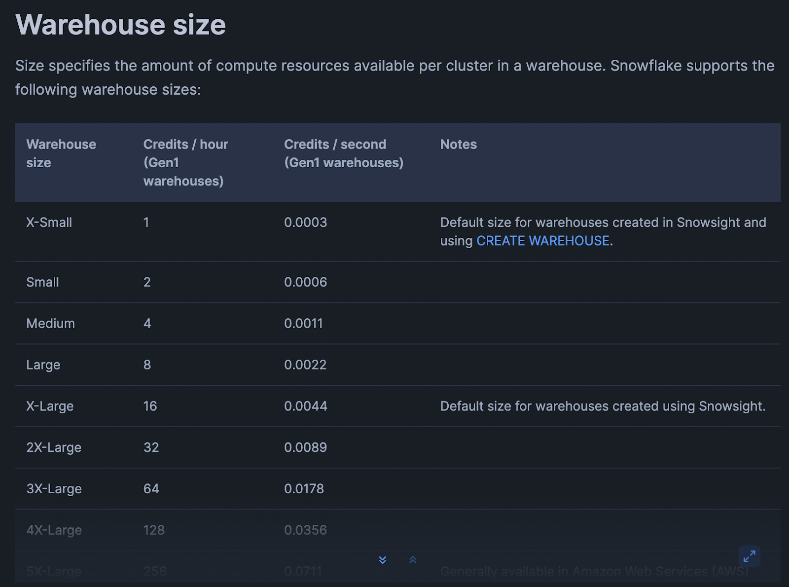
• Warehouse size (XS, S, M, L, XL, etc.)
• Time the warehouse is running (per-second, with a minimum)
• Credits consumed per hour for that size

Conceptually: Credits used = (credits/hour for size) × (seconds running / 3600)

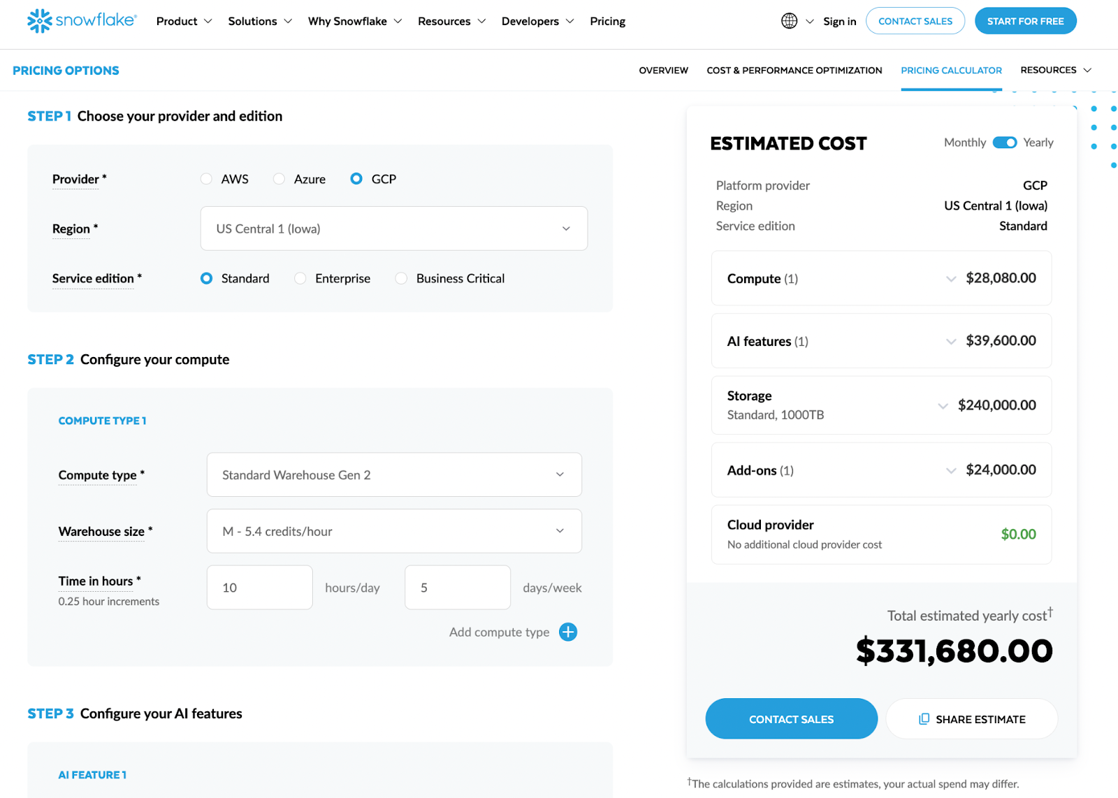
Example (numbers for illustration, check your account/edition for exact rates):

• XS warehouse: 1 credit/hour
• S warehouse: 2 credits/hour
• M warehouse: 4 credits/hour

If an XS warehouse runs for 15 minutes: 1 credit/hour × (900 seconds / 3600) ≈ 0.25 credits

If an M warehouse runs for the same 15 minutes: 4 credits/hour × (900 / 3600) ≈ 1 credit

Same duration, 4x the credits. That multiplier applies to every BI refresh, every ad-hoc query, every batch job that touches that warehouse.

Important mechanics to keep in mind:

1. Per-second billing, but minimum charge windows: Snowflake charges per second, but there’s a minimum (e.g., 1 minute) after each resume. Constantly starting and stopping warehouses can lead to paying these minimums repeatedly.
2. Auto-suspend and auto-resume

• Auto-suspend defines how long of inactivity before the warehouse stops billing.
• Auto-resume means the first query after suspend restarts the engine.
  Poorly tuned settings mean warehouses idle for minutes between sporadic dashboard queries, silently burning credits.

3. Multi-cluster warehouses: when concurrency is high, Snowflake can spin up additional clusters for a single warehouse. That increases credits consumed because you’re now paying for multiple clusters in parallel.

What matters in practice isn’t just how many queries you run, but how long warehouses remain active to support sporadic, overlapping workloads.

Warehouse Sizes, Concurrency, and Why Bigger Is Not Always Better

When dashboards are slow or large transformations lag, the default reaction is often: “Let’s bump the warehouse size.” This works – but it’s rarely cost-neutral.

Key trade-offs:

(1) Larger warehouse = faster queries, more credits per second: Scaling up from S → M may cut query time roughly in half but double your burn rate per second. If queries don’t actually speed up proportionally, you’re just paying more for similar latency.

(2) Concurrency vs. size. Warehouses handle a certain level of concurrency (simultaneous queries) before queuing:

• A bigger warehouse can process more work in parallel per cluster.
• A multi-cluster setup can also handle more concurrency without queuing, by adding clusters.
  Both increase potential throughput but also the maximum rate at which you burn credits.

(3) Underutilized big warehouses
A large warehouse serving spiky workloads (e.g., a few heavy queries every 10 minutes) can sit mostly idle and still burn credits. You’re paying for peak capacity, not average load.

Examples:

• A BI warehouse upgraded from S → L “to make dashboards snappy”:
  
  • Peak hour performance improves.
  • Off-peak, only a couple of queries per minute hit the warehouse.
  • Auto-suspend is set to 15 minutes “just in case” – so the L warehouse sits idle frequently, burning credits at L rates.
• A shared “ANALYTICS_WH” serving ETL, ad-hoc, and BI:
  
  • Concurrency spikes trigger multi-cluster scaling.
  • ETL jobs, exploration, and dashboards compete for capacity, pushing Snowflake to run more clusters.
  • Credits skyrocket during business hours, even though each individual workload looks “reasonable.”

Bigger warehouses and multi-cluster configs are powerful tools. But without clear separation of workloads and governance, they often become blunt instruments that increase your spend faster than your agility.

How BI Tools, Dashboards, and Connectors Translate Into Compute Usage

Most analytics teams don’t write SQL directly against Snowflake all day. Instead, they use BI tools and connectors that generate SQL for them. Understanding how those tools behave is critical for decoding your compute bill

Live connections

Tools like Looker Studio, Power BI (DirectQuery), Tableau live connections, and many reverse-ETL connectors send queries directly to Snowflake whenever:

• A user opens a dashboard.
• A filter or parameter is changed.
• A scheduled refresh kicks in.

Each such interaction results in one or more SQL queries that:

• Run on a specific warehouse.
• Trigger auto-resume if the warehouse is suspended.
• Keep the warehouse active until auto-suspend kicks in.

Scheduled dashboard refreshes

Dashboards are often configured to refresh:

• Every 5–15 minutes for “real-time” views.
• On business hours schedules (e.g., 8:00–20:00, Monday–Friday).

If each refresh runs the same complex queries against raw or semi-modeled data, you’re effectively running an ETL job many times per hour – but wrapped inside a BI tool.

Connector behavior

Some tools (reporting platforms, sync tools, embedded analytics, etc.) may:

• Issue multiple near-identical queries to build different widgets.
• Re-fetch the same aggregates instead of caching them.
• Use “SELECT *” on large tables to simplify mapping logic.

All of this translates into extra seconds (or minutes) of warehouse run time and additional credits.

Scenario -  main marketing kpi dashboard:

• Refreshes every 10 minutes from 8:00–20:00 (72 refreshes/day).
• Each refresh triggers 5 heavy queries hitting a campaign_events table with tens of millions of rows.
• Warehouse is an M, auto-suspend set to 15 minutes.

Result:

• Warehouse rarely suspends during business hours.
• You’re effectively running an M warehouse for 12 hours/day just for this dashboard, even if user traffic is light.

This is where well-designed aggregated Data Marts (exposed to BI tools) can drastically reduce compute: BI sends simple queries to small, pre-aggregated tables instead of re-computing complex joins each time.

Common Reporting Patterns That Multiply Snowflake Credits

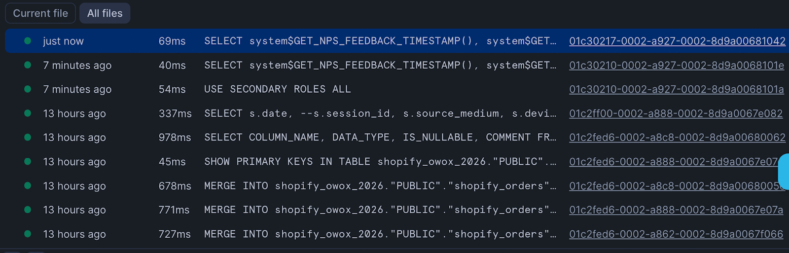
When you look at your Snowflake history, you’ll often see hundreds or thousands of similar queries. Individually they look cheap. Collectively, they dominate your spend on Snowflake infrastructure…

‍

Some typical patterns:

1. Duplicated SQL across dashboards and tools

• The same customer LTV calculation implemented in multiple dashboards, each executing its own heavy query chain.
• KPI logic copied into ad-hoc notebooks, internal tools, and external-facing analytics.

Every copy of that logic means another set of queries scanning base tables instead of reading from a shared, pre-computed mart.

2. Multiple BI tools hitting the same raw data

• Marketing uses Tool A, Product uses Tool B, Finance uses spreadsheets via ODBC.
• All connect live to Snowflake and query the same large fact tables.
• Each team rebuilds similar aggregates independently.

From Snowflake’s perspective, this is just more concurrent queries against the same warehouse, potentially triggering multi-cluster scaling.

3. Overly broad queries

• “SELECT *” on large event or clickstream tables to power BI, even if only a handful of columns are used.
• No date filters or partitions, scanning years of data for a last-30-days dashboard.

These choices increase scan time and warehouse runtime, particularly on larger warehouse sizes.

4. Excessive auto-refresh

• Dashboards set to 1–5 minute refresh intervals “just in case” someone is looking.
• Connectors that poll frequently for changes even when data updates are hourly or daily.

Each refresh reopens the warehouse window and extends its active period.

5. Lack of Data Marts

• Without a data mart layer, every team builds their own views, each with joins across raw fact and dimension tables.
• Heavy logic (e.g., attribution, cohorting) is re-executed in every context.

In contrast, a centralized data mart approach – maintained by your data team or via a solution like OWOX Data Marts – concentrates heavy transformations into scheduled jobs. BI then runs lightweight selects against these pre-computed tables, dramatically reducing per-query cost.

‍

Once you recognize these patterns, you can start designing around them: right-size warehouses for reporting, separate workloads, and introduce governed Data Marts to centralize heavy logic. In the next sections, we’ll connect these insights directly to architecture decisions that make your Snowflake costs both understandable and predictable.

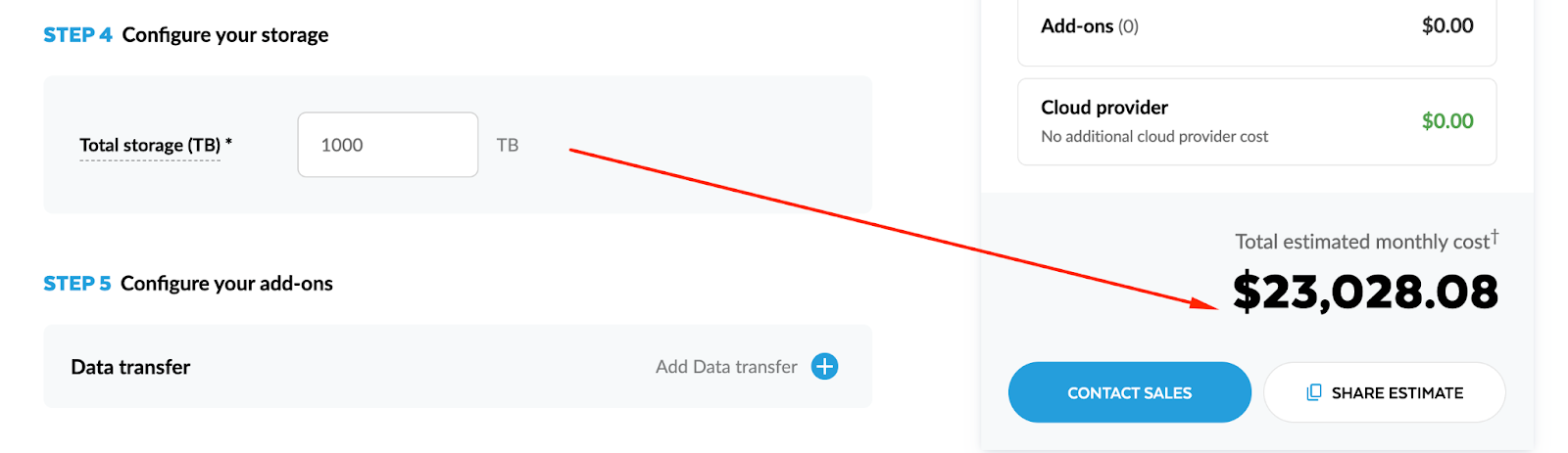
Snowflake Storage and Data Transfer: Predictable Costs with Architectural Traps

Compared to compute, Snowflake storage and data transfer costs look calm and predictable. Storage grows with your data volume; transfer grows with how much you move out. There are clear price-per-TB and price-per-GB numbers, and they don’t spike just because somebody opened a dashboard too many times.

However, architectural choices can multiply these “stable” components quietly in the background. Excessive raw data duplication, overly generous time travel policies, or fragmented reporting across regions and tools can turn a predictable line item into a creeping liability.

What Snowflake Storage Pricing Actually Covers and Why It Is Usually Stable

Snowflake storage pricing is primarily about how many compressed terabytes you keep in the platform over time. The mechanics are simple:

You pay for:

1. Table data

• Permanent, transient, and temporary tables (with different retention behaviors).
• Micro-partitions storing your actual data.

2. Time Travel and Fail-safe data

• Past versions of tables kept for recovery and audit.
• Snowflake-managed fail-safe copies after time travel expires.

3. Internal stage data

• Files temporarily stored during loads/unloads (depending on usage).

In many mature Snowflake environments, storage is a smaller and much more stable part of the bill than compute. That said, a few design choices can push it higher than it needs to be.

Storage pricing facts:

• Storage is charged per TB per month, based on average volume.
• Compressed size matters more than raw file size.
• Long retention + aggressive duplication can compound quickly.

Time Travel, Fail-safe, and The Impact of Raw Data Duplication

Snowflake’s resilience features are powerful, but they’re not free.

Time Travel & Fail-safe

• Time Travel lets you query historical versions of tables for a configurable retention window (e.g., 1–90 days depending on edition and table type).
• Fail-safe extends recoverability beyond Time Travel, managed automatically by Snowflake.

Cost implications:

• The longer your Time Travel retention, the more historical data Snowflake keeps around.
• Every schema change, delete, or overwrite creates new versions that are retained for that period.
• Fail-safe adds a small additional footprint after Time Travel expires.

For analytics workloads, this is often worth the cost – but defaulting to maximum retention everywhere can bloat storage unnecessarily.

Raw data duplication

The bigger trap is uncontrolled duplication of raw datasets:

1. Multiple “raw” schemas or databases

• Ingesting the same source (e.g., events, CRM, ads) into multiple raw areas for different teams or environments.
• Copying raw tables instead of referencing them or using views.

2. Environment sprawl

• Full copies of production data into dev, staging, QA, sandbox, and “backup” databases.
• Keeping those copies around indefinitely.

3. Snapshot-heavy data modeling

• Naively snapshotting entire tables daily (or more often) without pruning or partitioning.
• Storing each snapshot as a full copy, not as incremental deltas.

Storage line items from these patterns won’t jump overnight, but they will:

• Grow steadily and quietly.
• Make it harder to reason about which datasets are truly needed.
• Increase the impact of long Time Travel windows.

A disciplined approach to raw data (one canonical raw layer, deliberate environments, controlled snapshot strategy) keeps storage behaving like the predictable cost center it should be.

When Reporting Architecture Breaks Your Snowflake Cost Predictability

If your Snowflake bill feels random month to month, the root cause is almost never “mysterious pricing.” It’s usually your reporting architecture.

The way metrics are defined, how BI tools connect, where SQL lives, and how self-service is enabled all determine how often and how heavily you hit your warehouses. That’s what drives compute spikes – not the fact that you have 10 TB or 50 TB of data sitting in storage.

Metrics and Logic Defined In Dashboards Instead of Governed Data Marts

In many organizations, business logic lives where it’s most convenient at the moment: inside BI dashboards, notebook cells, or even spreadsheet formulas. The same KPI (say, “Active Customers”) might be implemented differently in:

• The marketing dashboard
• The product analytics dashboard
• A finance spreadsheet
• A leadership slide deck data source

From a Snowflake cost perspective, this has two major effects:

1. The same heavy calculation is re-run many times

• Each dashboard defines its own SQL to compute Active Customers from raw events, orders, and CRM tables.
• Every time one of these dashboards refreshes, Snowflake recomputes those joins and aggregations from scratch.

2. Complex queries run closer to the BI layer, not in a reusable data mart environment

• Instead of hitting a compact data_mart_customers_active table, BI sends big, complex queries to raw or lightly-modeled tables.
• These queries are more expensive, take longer, and keep warehouses active longer.

Scenario:

• Marketing defines CAC, LTV, and churn in a Looker explore.
• Product defines them separately in a different tool.
• Finance has their own SQL in a spreadsheet connector.

Each definition:

• Hits the same base tables (events, subscriptions, payments) independently.
• Generates long-running queries during dashboard refreshes and monthly reporting.
• Multiplies compute usage for logic that should be centralized once.

A governed Data Mart layer solves this by:

• Implementing KPIs centrally (e.g., dm_customer_metrics_daily).
• Letting dashboards query lightweight aggregates instead of reconstructing business logic on every view.

Solutions like OWOX Data Marts are built around this idea: metrics live in marts, not in dashboards, so you compute once and reuse everywhere.

Per Report and Per Team SQL Duplication Across BI Tools and Sheets

SQL duplication is another silent cost amplifier. It happens when every team, and sometimes every analyst, writes their own version of similar queries. Common patterns:

Per-report SQL

• Each new dashboard or report gets its own queries, even if it shows the same KPIs with slightly different filters.
• Queries are copy-pasted with small modifications, then evolve separately.

Per-team logic forks

• Marketing builds its own “attribution” logic in Tool A.
• Product builds its own retention and activation logic in Tool B.
• Data Science builds a third set in notebooks, exported back to Snowflake.

Apps Script & custom connectors

• Analysts build sheets that connect directly to Snowflake and embed SQL in the connection.
• Those sheets are shared and cloned across teams, multiplying the number of near-identical queries that run regularly.

Example

• You have 5 major departments, each with their own BI environment.
• Each defines a monthly revenue breakdown report.
• All of them independently run multi-join SQL against orders, line_items, discounts, and currency_rates.

Result?

• 5× the compute for almost the same result set.
• Bursts of load during closing periods as each team runs its reports.

With centralized Data Marts (dm_revenue_monthly, dm_revenue_by_channel), all those reports can issue simple selects against pre-aggregated data. Compute shifts from “many scattered, redundant queries” to “a few controlled, scheduled jobs.”

Uncontrolled Self-service and Live Connections That Hammer Warehouses

Self-service analytics is a goal for most data teams – and Snowflake plus modern BI tools make it extremely easy to achieve. The risk is when “self-service” means “no governance.”

Symptoms of uncontrolled self-service analytics:

1. Too many users with direct access to raw or lightly-modeled schemas
2. Live connections everywhere
3. No workload separation

Real impact on consumed credits:

• A single exploratory session by an analyst might run tens of ad-hoc queries, each scanning millions or billions of rows.
• A popular dashboard with live connection and low auto-refresh interval effectively keeps a warehouse running all day, even when very few people are actively using it.
• During high-usage weeks (campaign launches, product releases, quarter-end), self-service usage can double or triple, causing noticeable cost spikes.

Example:

• 30 self-service users across marketing and product.
• Each builds their own funnel, retention, and cohort analyses on raw events.
• They use a live-connected BI tool, refreshing dashboards every 5 minutes.

Result:

• The analytics warehouse is almost never suspended during business hours.
• Multi-cluster kicks in during peak times as users explore in parallel.
• Credits consumed per day are much higher than the “core” scheduled workloads would suggest.

Self-service analytics is valuable – the problem is where it points. 

Pointing it at raw data guarantees unpredictable compute. Pointing it at governed Data Marts still gives flexibility, but against pre-aggregated, cost-efficient tables.

A Governed Data Mart Layer on Snowflake as the Foundation for Cost Control

Once you understand that compute spend is driven by how you query Snowflake, not just how much data you store, the natural next question is: where should business logic live so that queries are efficient and reusable?

The answer, for most analytics teams, is a governed Data Mart layer on top of Snowflake. This is the architectural piece that turns a powerful warehouse into a predictable analytics platform – one where metrics are consistent, self-service is safe, and compute costs don’t explode when more people start asking questions.

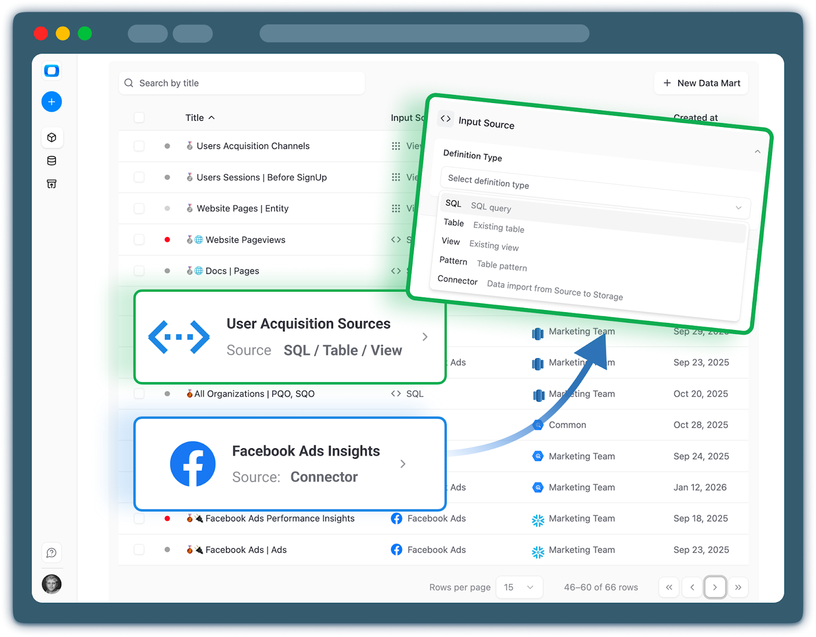
What a Snowflake Data Mart Is and How It Differs From Raw Tables

A Data Mart in Snowflake is a curated, SQL- or table-defined designed specifically for analytics and reporting and answering a specific business question. 

It sits on top of your raw (bronze) and modeled (silver) layers of data and presents business-ready structures to BI tools and stakeholders / end users.

Key characteristics of a Data Mart:

1. Business-oriented

• Data Marts are organized around domains (e.g., dm_marketing_performance, dm_product_usage, dm_revenue) rather than source systems.
• Columns are named in business language, not internal API fields.

2. Pre-aggregated and denormalized where it matters

• Common joins and aggregations are materialized.
• BI and analysts query compact, analytics-friendly tables instead of stitching together raw sources.

3. Governed and versioned

• Owned by data analysts with clear ownership & management.
• Metrics definitions are documented.

‍

IMPORTANT!
How this differs from raw tables:

• Raw tables reflect the structure of source systems (events, logs, CRM exports). They’re optimized for ingestion, not consumption.
• Data Marts reflect the structure of business questions (funnels, revenue, retention). They’re optimized for repeated reads.

In other words, a Data Mart is the contract between your complex backend data and your many front-end tools and stakeholders.

Defining Metrics Once and Reusing Them Across Teams and Tools

One of the main drivers of unpredictable compute is metrics logic scattered across dashboards, queries, and notebooks. Data Marts invert this pattern by making metrics a first-class, centralized asset.

In a governed mart layer - Metrics are encoded. BI tools read, they don’t redefine. Teams consume the same definitions. Marketing, Product, Finance, and Leadership all pull from the same metric tables. This eliminates “multiple truths” and reduces the temptation to clone or rewrite metric logic.

Benefits:

• Consistency: A “conversion rate” chart means the same thing across tools.
• Maintainability: Data engineers can improve logic or fix bugs in one place.
• Cost predictability: Heavy calculations are centralized in scheduled mart builds, not re-executed every time someone opens a dashboard.

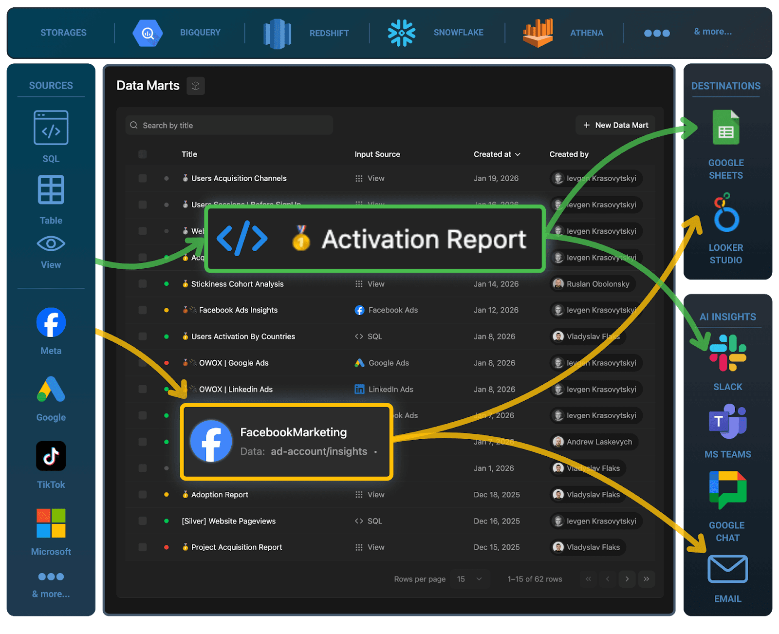
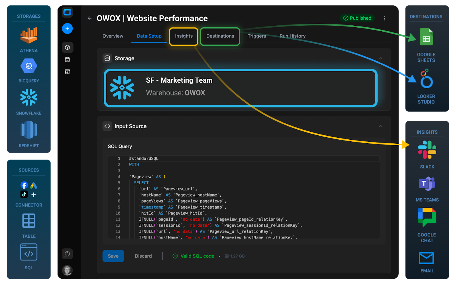
Platforms like OWOX Data Marts are built exactly around this principle: define metrics once in a governed layer, then surface them uniformly to Looker, Power BI, Google Sheets, or any other consumer.

Keeping Snowflake as the System of Truth While Enabling Safe Self-service Analytics

A common fear is that introducing a governed mart layer will slow teams down or centralize too much control in the data team. The reality is the opposite if you design it well.

With governed Data Marts:

Snowflake remains the system of record

Raw data, intermediate models, and marts all live in Snowflake. There’s no need to export full datasets into external engines just to make reporting work.

Self-service operates on safe, curated surfaces

Business users and analysts can freely explore mart schemas without fear of “breaking the warehouse.” They work with stable, documented tables that are designed for exploration.

Permissions are simpler and safer

Access policies can be defined at the mart schema level, instead of exposing sensitive raw tables. This reduces the risk of leaking PII or internal operational details.

Governance and agility coexist

The data team owns the contract: which marts exist, what fields mean, how often they’re refreshed. Within that contract, teams can build whatever dashboards, reports, and ad-hoc analyses they need.

From a cost-control standpoint, this balance is powerful:

• You encourage self-service on top of marts, where queries are cheap and predictable.
• You constrain direct access to raw/volatile layers, where queries are expensive and unpredictable.

If you don’t want to build this entire data mart layer and governance machinery yourself, just start using OWOX Data Marts right now. 

The end result: Snowflake stays your single source of truth, while the Data Mart layer becomes the “shock absorber” between complex backend data and messy real-world reporting needs – smoothing out both your analytics experience and your monthly compute bill.

Putting It All Together: A Snowflake Cost Control Strategy Built on Governance

Snowflake pricing isn’t the real problem. The real problem is when reporting architecture and workflows are left to grow organically – with metrics in dashboards, duplicated SQL, and live connections pointing at raw data.

Controlling cost means governing how Snowflake is used: centralizing business logic, batching heavy computation, and exposing safe, reusable Data Marts to all your tools. Use this section as a practical blueprint to assess where you are and what to do next.

Checklist to Assess Whether Reporting Architecture Is Driving Your Snowflake Bill

Use this checklist to quickly spot if your reporting layer is the main driver of your Snowflake compute spend:

Dashboards & BI

• Many dashboards and reports define metrics (LTV, ROAS, churn, funnels) directly in BI tools

• Multiple BI tools (and/or Google Sheets) connect live to Snowflake

• Dashboards refresh every 5–15 minutes, even for daily or weekly metrics

• The same KPI appears in several dashboards, each powered by different SQL

SQL & Data Modeling

• SQL for core metrics is copy-pasted across tools, notebooks, and sheets

• Teams query raw or lightly-modeled tables directly for reporting

• There’s no clear “analytics-ready” mart schema for each domain (marketing, product, finance)

• You can’t easily list where a given business metric is defined

Warehouse Behavior

• Reporting warehouses are oversized “just to keep dashboards fast”

• Warehouses rarely auto-suspend during business hours

• Concurrency spikes (month-end, campaigns) force you to scale up or enable multi-cluster

• Finance sees compute consumption jump whenever new dashboards or tools are rolled out

If you checked several of these, your Snowflake costs are likely a workflow and governance issue, not a pricing or storage problem.

How to Pilot OWOX Data Marts on One Domain Before Scaling

If you’d rather not build orchestration, monitoring, and connectors yourself, you can pilot OWOX Data Marts on a single domain and expand from there. Suggested pilot approach:

1. Connect Snowflake to OWOX as a Storage
2. Choose one high-impact domain (Marketing is a common first candidate (ads, web analytics, revenue attribution). Alternatively, pick product analytics or core revenue reporting – wherever dashboards are most painful and costs most visible.
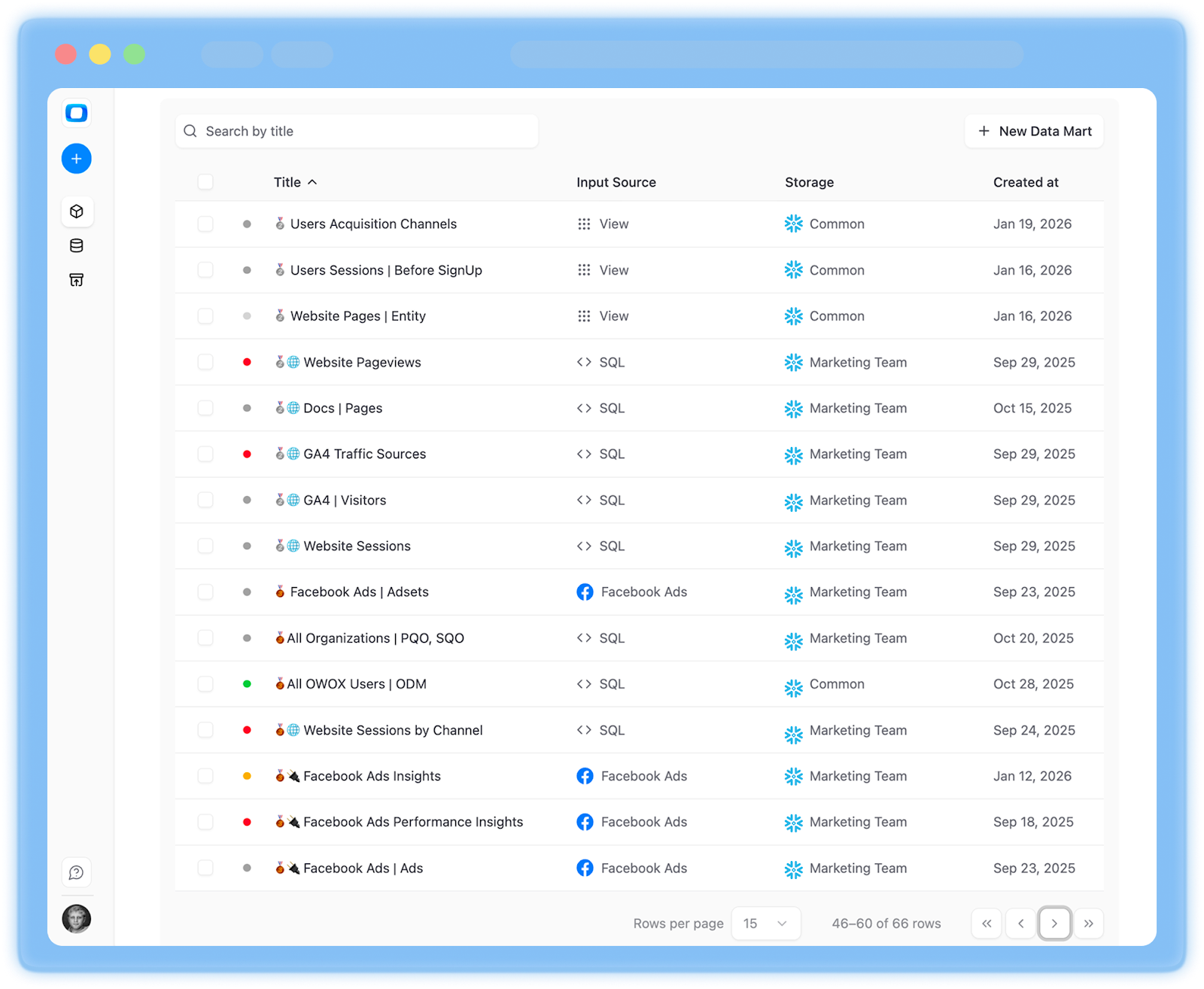
3. Use OWOX to define the first data mart. Start with out-of-the-box templates or write your own SQL in OWOX. Implement 2–5 key data marts (e.g., traffic, spend, attribution, ROAS).
4. Connect Google Sheets & set refresh schedules 
5. Share those reports with business users and see how your value & impact grows in 2-4 weeks

Once you’re confident in the pattern, you can replicate it across other domains with much less friction.

OWOX Data Marts makes this layer practical to implement and operate on top of your existing Snowflake setup. You keep Snowflake as your system of truth; OWOX turns it into a governed, efficient reporting platform. You can start with a single domain, see the impact on performance and cost, and expand once it proves its value.

Get started for free and see how much more predictable your Snowflake bill can be…