
Mastering the TEXT Function in Google Sheets: Formatting Made Simple
Master the TEXT Function in Google Sheets to format data, customize text, and enhance presentation for seamless readability.


Efficiency in spreadsheet management often hinges on the ability to customize text formatting precisely. The TEXT function in Google Sheets is a powerful tool that simplifies this process, allowing you to format numbers, dates, and other data types into readable text formats with ease.
Whether you need to display currency, percentages, dates in a specific style, or any other data customization, the TEXT function offers a flexible solution.
This guide will take you through the essentials of using the TEXT function, providing practical examples to show how it can transform your data presentation and enhance your spreadsheet’s functionality. Learn to leverage this function to make your data not only more visually appealing but also more functionally organized and accessible.
The Importance of Data Cleanup for Google Sheets Users
For Google Sheets users, data cleanup is paramount. It ensures the accuracy, consistency, and reliability of your data, reducing errors in your analysis and facilitating better decision-making. Moreover, clean data not only saves time but also presents a more professional appearance, especially when you need to showcase your findings to others.
Whether you're formatting with the TEXT function or employing other tools, proper data cleanup is a crucial step that enhances the overall quality and effectiveness of your work in Google Sheets.
Exploring the TEXT Function (With Syntax and Examples)
Hone your text management skills in Google Sheets with essential functions like TEXT, which customizes formatting to suit your needs. Below, we will explore the syntax and examples of the TEXT function, demonstrating its versatility in enhancing your data cleaning and formatting capabilities. This guide will help you master the art of text manipulation, making your spreadsheets more efficient and your data presentation more effective.
TEXT Function
The TEXT function in Google Sheets is beneficial for ensuring report consistency, making raw data more presentable, and aligning it with specific formatting requirements.
Syntax of TEXT
=TEXT(number, format)
Let's break down the parameters:
- number: The numeric value, date, or time you want to format.
- format: A string enclosed in quotation marks that specifies the desired format.
This is particularly useful for displaying numbers more readably or standardized, such as formatting dates, times, or currency values.
Example of TEXT
Let’s say you have Price data in column C. You want to format the prices to display one decimal place for better readability.
Syntax:
=TEXT(C4, "0.0")
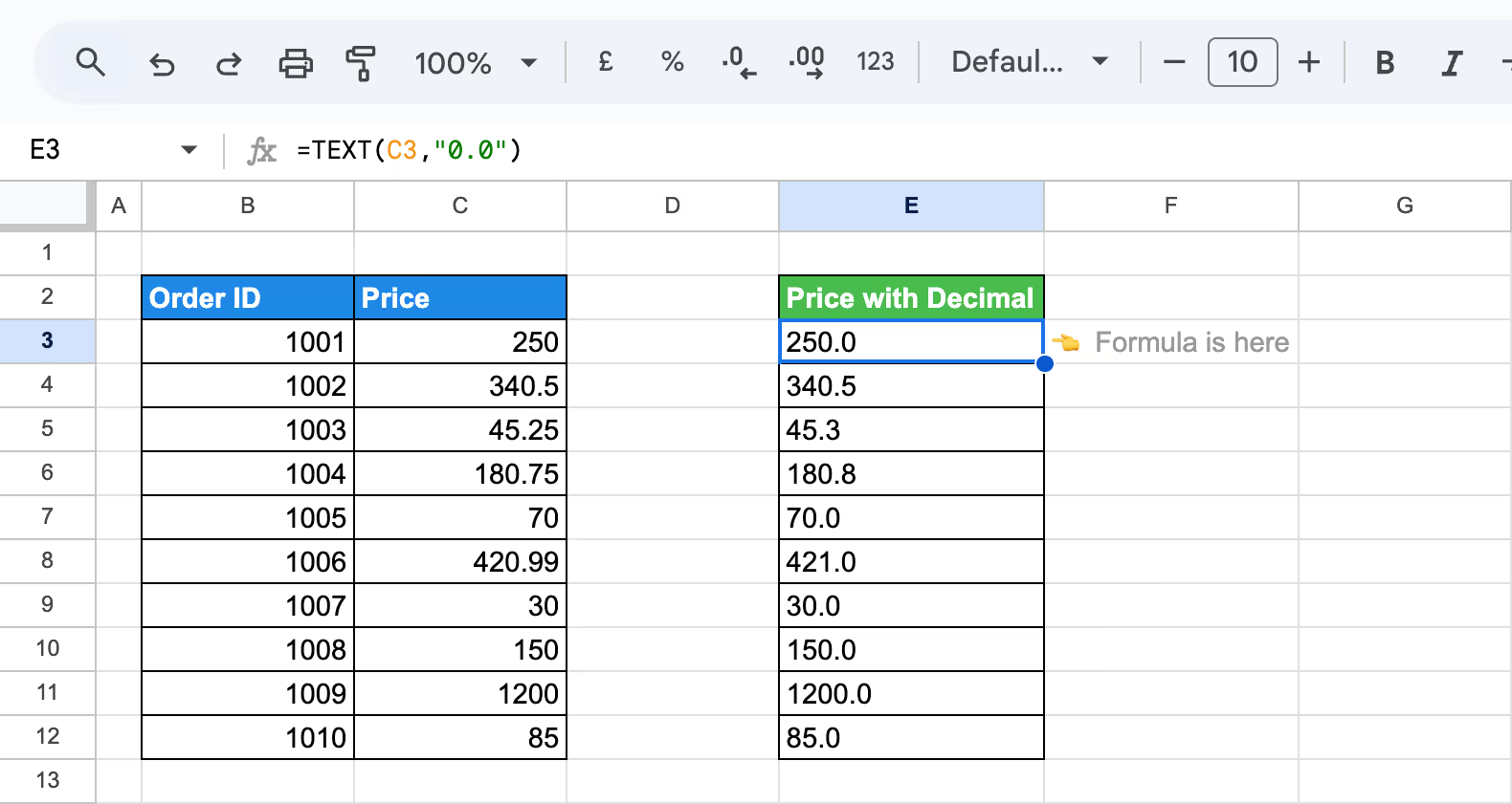
Here:
- C4: Refers to the price value in column C.
- "0.0": Ensures the price is displayed with one decimal place.
The formula converts the numbers in column C to text format with consistent decimal precision, as shown in column E.
Simple Examples of Using TEXT Function in Google Sheets
The TEXT function in Google Sheets simplifies data handling by allowing you to format dates and other values precisely to your needs. This versatile tool can streamline your tasks and enhance your spreadsheet workflows. In this section, we'll provide simple examples to demonstrate how the TEXT function works and how it can improve your data management practices, making your spreadsheets more functional and your data more presentable.
Transforming Date Formats with the TEXT Function
The TEXT function in Google Sheets is a versatile tool for reformatting dates, making your dataset consistent and presentation-ready. By applying a specific format, such as "mm/dd/yyyy," you can standardize reports, analysis, or collaboration dates.
Example:
Let’s say you have Order Dates in column C and need to convert them to the "mm/dd/yyyy" format.
Use the following formula in a new cell:
=TEXT(C3, "mm/dd/yyyy")
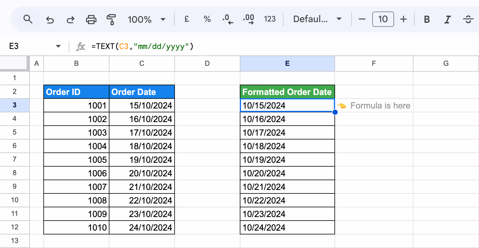
Here:
- C3: Refers to the cell containing the original date.
- "mm/dd/yyyy": Specifies the desired date format.
This formula reformats the Order Dates in column E, ensuring uniform and easily readable dates throughout the dataset.
Merging Text and Numbers Seamlessly with TEXT
The TEXT function in Google Sheets makes it easy to merge text and numbers while preserving formatting. This function ensures that numerical values are displayed in the desired format, such as dates, currency, or percentages, when combined with text, providing seamless and consistent data presentation.
Example:
Let’s say you have Order ID data in column B and want to append the phrase "Order ID:" before each number.
Use the following formula in a new cell:
="Order ID: "&TEXT(B3, "0")
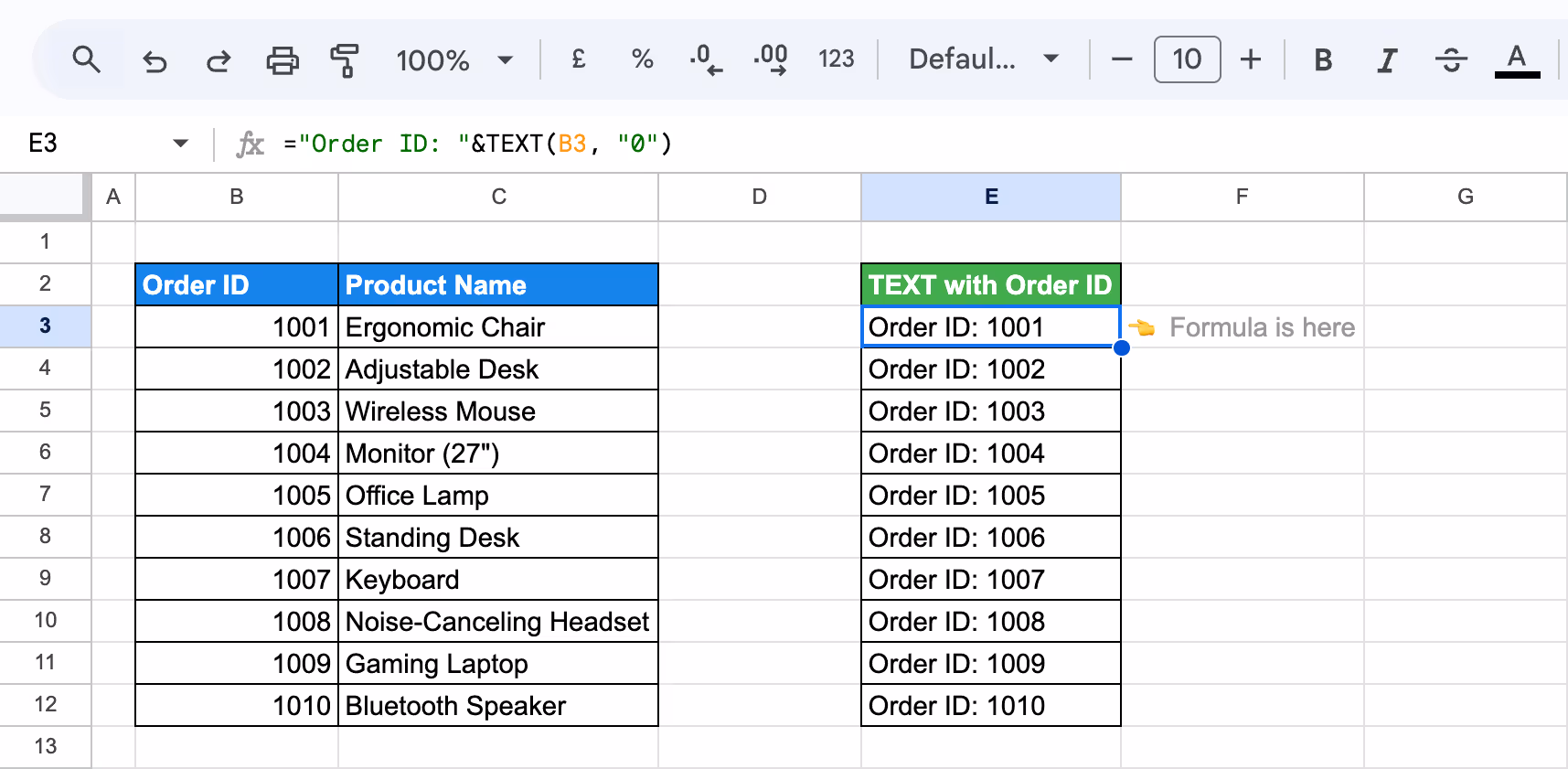
Here:
- B3: Refers to the cell containing the Order ID number.
- "0": Ensures the number is formatted as a whole number.
This formula combines the text "Order ID:" with the formatted Order ID in column B, producing a clear and readable result in column E.
Converting Values into Currency Formats Using TEXT
The TEXT function in Google Sheets simplifies formatting numerical values into currency formats. It ensures consistency and clarity by displaying numbers as formatted currency values. This is especially useful for creating professional reports, invoices, or financial summaries where clear monetary representation is essential for better understanding and presentation.
Example:
Let’s say you have raw price data in Column C. You want to format it as currency in Column E.
Use the following formula in a new cell:
=TEXT(C3, "$#,##0.00")

Here:
- C3: Refers to the cell containing the price value.
- "$#,##0.00": Converts the number into a currency format with two decimal places.
The resulting values in column E, like "$250.00" and "$1,200.00," make the dataset visually appealing and easy to interpret for financial reports or presentations.
Representing Decimals as Percentages with TEXT
The TEXT function in Google Sheets allows you to seamlessly merge text and numbers, ensuring clarity and consistency in your data. It’s handy for creating descriptive outputs, such as appending labels or phrases to numbers, formatting them for readability, and making datasets easier to interpret.
Example:
Let’s say you have decimal values in column C and want to display them as percentages in column E. Using the formula ensures values like 0.1 appear as "10%" and 0.05 as "5%."
Use the following formula in a new cell:
=TEXT(C3, "0%")

Here:
- C3: Refers to the cell containing the decimal value.
- "0%": Formats the decimal into a percentage representation.
The percentages in column E improve data clarity, making it suitable for reports and easy interpretation.
Advanced Examples of Using TEXT Function in Google Sheets
Expanding beyond the fundamentals, this section showcases advanced examples that illustrate the power of combining the TEXT function with other formulas for sophisticated tasks.
Whether you're creating custom formatting for dynamic reports, cleansing datasets for precise analysis, or generating specific patterns or placeholders, these examples highlight the TEXT function's adaptability in managing complex spreadsheet operations effectively.
Creating Custom Number Formats with TEXT
The TEXT function in Google Sheets allows you to create custom number formats effortlessly. By combining numbers with specific text or symbols, you can present data like quantities, percentages, or currencies in a clear, readable way. This enhances data interpretation and ensures professional formatting in reports or dashboards.
Example:
Let’s say you have order quantities in column C, and you want to display them in Column E with "units" for clarity.
Use the following formula in a new cell:
=TEXT(C3, "###0") & " units"
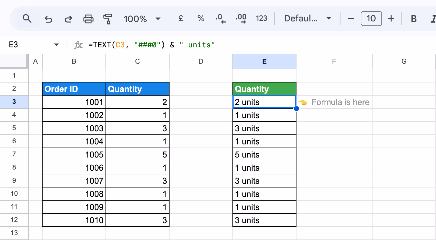
Here:
- C3: Refers to the cell containing the quantity.
- TEXT(C3, "# ##0"): Ensures the number is displayed without decimals.
- & " units": Concatenates the formatted number with the text "units."
This formula transforms numerical values in Column C into a readable format in Column E, such as "2 units" or "1 unit," enhancing data presentation for reports or records.
Advanced Time Formatting with TEXT
The TEXT function in Google Sheets allows you to convert raw time values into formats like hh:mm AM/PM or hh:mm:ss, enhancing data readability. It’s ideal for presenting schedules, timelines, or logs in a user-friendly and visually appealing manner.
Example:
Let’s say you have an Order Time dataset in column C and want to convert it to a more readable "h:mm AM/PM" format in column E.
Use the following formula in a new cell:
=TEXT(C3, "h:mm AM/PM")
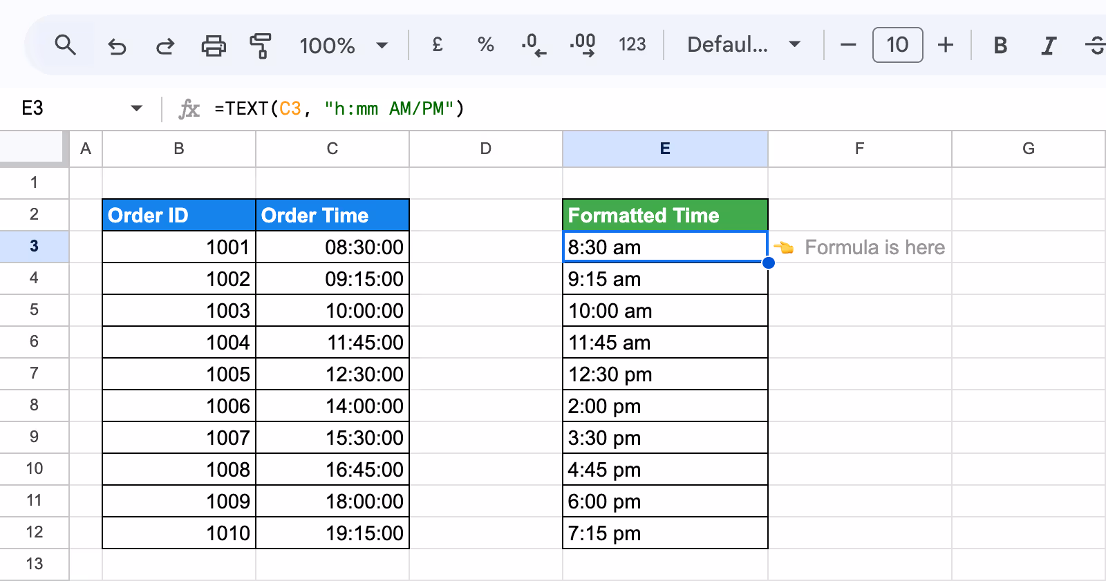
Here:
- C3: Refers to the cell containing the original time.
- "h:mm AM/PM": Converts the time to a 12-hour clock format with AM/PM notation.
This formula transforms time values in column C into a user-friendly format, like "8:30 am" or "2:00 pm," improving readability for schedules or reports.
Combining TEXT Function with Other Functions
Integrating the TEXT function with other Google Sheets functions can greatly improve your data cleaning and analysis processes. This combination enables more sophisticated operations, aiding in the optimization of workflows and the maintenance of accurate, consistent datasets throughout your spreadsheets.
This section will explore how to effectively harness the TEXT function alongside other tools to enhance your data management strategies.
Using TEXT with CONCATENATE for Combining Text and Values
Combining text and numerical values in Google Sheets can be easier with the CONCATENATE and TEXT functions. While CONCATENATE merges different text strings into one, the TEXT function ensures that numerical values are formatted according to your specifications, allowing for clear, readable outputs in reports or messages.
Example:
Let’s say you want to create a message showing each product's total purchases in a readable format.
Use the following formula in cell F2:
=CONCATENATE("Total purchases for ", C3, ": $", TEXT(D3, "#,##0.00"))
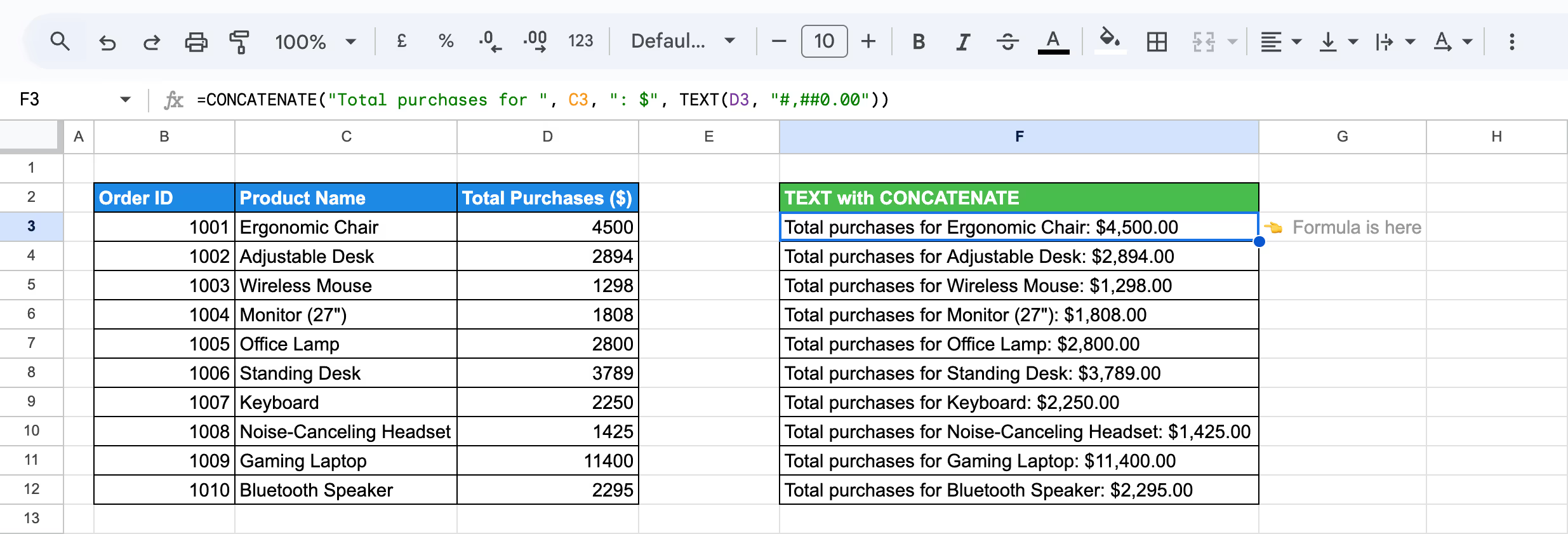
Here:
- CONCATENATE("Total purchases for ",C3, ": $"): Combines the product name from column C with the string "Total purchases for" and a dollar sign.
- TEXT(D3, "#,##0.00"): Formats the total purchases value from column D to show as currency, with two decimal places and commas for thousands.
- The CONCATENATE function: Combines these elements into a single text string, displaying the formatted output.
The result will return a message like "Total purchases for Ergonomic Chair: $4,500.00". Drag the fill handle down to apply the formula to other rows.
Formatting Dates with TEXT and DATE Functions
The TEXT and DATE functions are powerful tools for formatting and manipulating dates. Combining these functions allows you to display dates in various formats and create dynamic date values based on specific criteria.
Example:
Let’s say you have a dataset with order dates, and you want to format them to display in a more readable way, such as "October 15, 2024."
Use the following formula in cell
=TEXT(DATE(2024, 10, 15), "mmmm dd, yyyy")
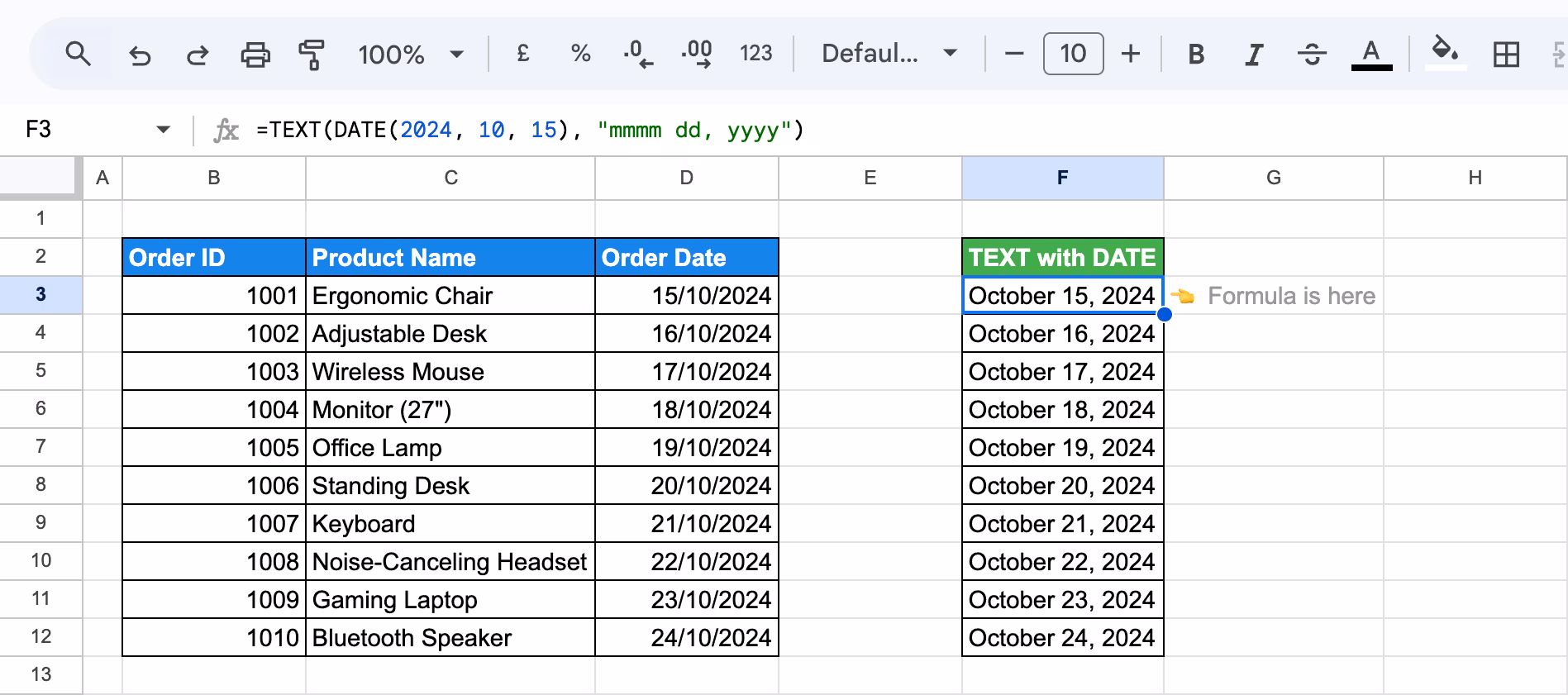
Here:
- DATE(2024, 10, 15): Converts the year, month, and day into a date value (October 15, 2024).
- TEXT(DATE(2024, 10, 15), "mmmm dd, yyyy"): The TEXT function then formats the date into "October 15, 2024" using the specified format "mmmm dd, yyyy."
By using the DATE and TEXT functions together, you can easily convert and format date values into more readable formats in Google Sheets.
Customizing Current Date and Time with TEXT and NOW
Using Current Date and Time with TEXT and NOW allows you to format the current date and time in a specific way using Google Sheets. By combining the NOW() function (which returns the current date and time) with the TEXT() function, you can display the date and time in custom formats.
Example:
Let’s assume new orders are coming in for specific products, and you need to inform customers immediately when their orders are dispatched. You decide to implement a Google Sheets workflow to capture this timestamp automatically. Let’s say you want to display the current date and time in a specific format, such as "November 24, 2024 12:59:00 PM."
Use the following formula:
=TEXT(NOW(), "mmmm dd, yyyy h:mm:ss AM/PM")

Here:
- NOW(): Returns the current date and time whenever the formula is recalculated.
- TEXT(NOW(), "mmmm dd, yyyy h:mm:ss AM/PM"): The TEXT function formats the current date and time into a custom format. In this case, it will display the date in "November 24, 2024" and the time in "1:07:10 PM".
The NOW() function always returns the current date and time when the formula is recalculated. The TEXT function allows you to customize the format to display it in a readable way.
Converting Summed Values into Custom Formats with TEXT and SUM
You can combine the SUM and TEXT functions to display the result of summed values in a specific format. This approach lets you calculate totals and format them according to your needs, such as showing the result in currency, percentages, or custom number formats.
Example:
Let’s say you have a dataset of product purchases. You want to sum the Total Purchases ($) and display the result in currency format, with commas for thousands and two decimal places.
Use the following formula in a new cell:
=TEXT(SUM(D3:D12), "$#,##0.00")

Here:
- SUM(D3:D12): Adds up all the values in the Total Purchases ($) column.
- TEXT(SUM(D3:D12), "$#,##0.00"): The TEXT function formats the summed value as currency with commas for thousands and two decimal places.
By combining SUM and TEXT, you can easily calculate totals and display them in a more readable and professional format, like currency, improving the clarity and presentation of your data.
💡 Looking to enhance your Google Sheets skills? Check out our article on SUM functions in Google Sheets to learn how to efficiently calculate totals, apply custom formats, and streamline your data analysis. Don't miss out on valuable tips and tricks! Read the full article here.


Formatting Averages Using TEXT and AVERAGE
Using the TEXT and AVERAGE functions allows you to calculate the mean of a range of values and display the result in a specific format, such as currency or with a set number of decimal places. This approach makes your data more readable and professional.
Example:
Let’s say you want to calculate the average Total Purchases ($) and format it as currency.
Use the following formula in the cell:
=TEXT(AVERAGE(D3:D12), "$#,##0.00")
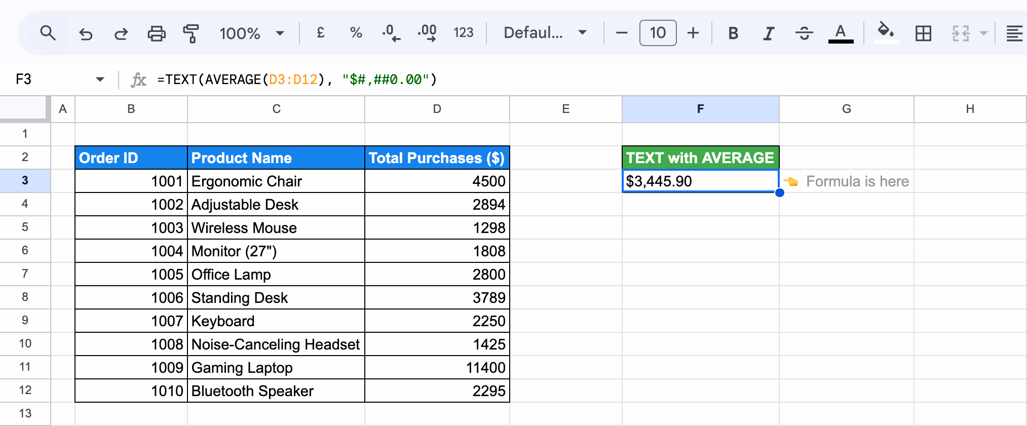
Here:
- AVERAGE(D3:D12): Calculates the average of the values in the Total Purchases ($) column).
- TEXT(AVERAGE(D3:D12), "$#,##0.00"): The TEXT function then formats this average as currency with commas for thousands and two decimal places.
Using TEXT and UPPER for Uppercase Conversion
Using the TEXT and UPPER functions allows you to convert text to uppercase. Combining these functions ensures that any text value is displayed in all capital letters, which helps standardize or emphasize specific data in your sheets.
Example:
Let’s say you have a list of Product Names in column C and want to display them in uppercase for consistency or to make them stand out in your report.
Use the following formula in the cell:
=UPPER(TEXT(C3, "0"))
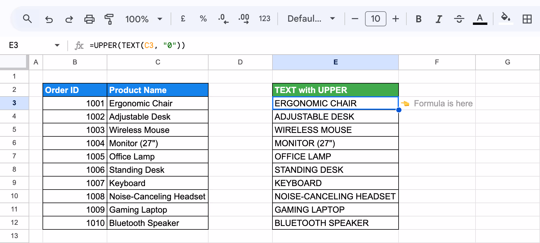
Here:
- TEXT(C3, "0"): Converts the value in cell (product name) to text.
- UPPER(TEXT(C3, "0")): The UPPER function then converts the resulting text into uppercase.
By combining TEXT and UPPER, you can quickly standardize and format your text data into uppercase letters, making it easier to maintain consistency across your dataset or improve report readability.
Combining TEXT with FIND and MID for Data Extraction
Combining the TEXT function with FIND and MID allows you to extract specific portions of text from a cell. This technique is useful when you need to isolate a substring, such as extracting product codes, names, or specific data from a larger string within your dataset.
Example:
Let’s say you want to extract the first name from the Customer Name column (Column C). To do this, you can use the FIND and MID functions in combination with TEXT.
Use the following formula:
=MID(TEXT(C3, "0"), 1, FIND(" ", TEXT(C3, "0"))-1)
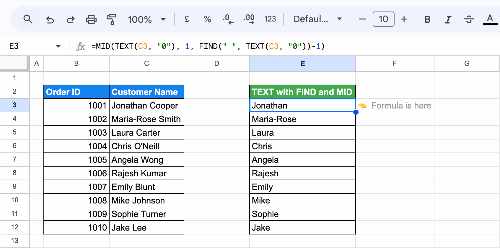
Here:
- TEXT(C3, "0"): Converts the Customer Name in cell C3 to text.
- FIND(" ", TEXT(C3, "0")): Finds the position of the first space in the name, which separates the first and last names.
- =MID(TEXT(C3, "0"), 1, FIND(" ", TEXT(C3, "0"))-1): Extracts the text starting from the first character and continuing up to the first space, essentially extracting the first name.
By combining the TEXT, FIND, and MID functions, you can easily extract specific portions of a text string, such as a first name from a full name.
Troubleshooting Common Issues with TEXT Function
While working with the TEXT function, you might come across errors like #VALUE!, #N/A, or #NAME. These issues often stem from using incorrect data types or from errors in function syntax. In this section, we will explore these common errors and provide guidance on how to resolve them effectively.
#VALUE! Error
⚠️ Error: The #VALUE! error with the TEXT function can occur when the format text is unrecognized, such as if the text isn't enclosed in quotation marks or the format code is incorrect.
✅ Solution: To fix this, make sure the format text in the TEXT function is properly enclosed in quotation marks and that the format codes are accurate (e.g., "dd/mm/yyyy" for dates). Verify each element to ensure compliance with the expected formatting standards.
#N/A Error
⚠️ Error: The #N/A error occurs when the input cell is empty, or the data cannot be found. This typically happens in functions like VLOOKUP or HLOOKUP when a match cannot be found for the specified lookup value.
✅ Solution: Ensure the cell you reference in your formula contains data. If the input cell is supposed to contain a date or time, verify that it is correctly formatted. Double-check the lookup values and ranges to ensure they match and contain valid data.
#REF! Error
⚠️ Error: The #REF! error occurs when an invalid cell reference is used in the formula. This can happen if you’ve deleted or moved cells that the formula previously referenced.
✅ Solution: Check your formula to ensure that all cell references are valid. Adjust your formula to reference the correct cells if you’ve recently deleted or moved cells. Double-check that no references point to deleted or shifted ranges.
#NUM! Error
⚠️ Error: The #NUM! error occurs when the formula results in a number too large or too small to be represented in Google Sheets.
✅ Solution: Review your formula to ensure it doesn't produce a result that exceeds the acceptable numerical range in Google Sheets. Adjust your formula or input data to avoid generating values that are too large or too small to be processed.
#DIV/0! Error
⚠️ Error: The #DIV/0! error occurs when a number is divided by zero in your formula. This typically happens when the denominator in a division operation is zero or an empty cell, which results in an undefined calculation.
✅ Solution: Review your formula to ensure that no division by zero is occurring. You can add a check to ensure the denominator is not zero before performing the division (e.g., using an IF statement or ISERROR). If necessary, adjust your formula or input data to prevent the divisor from being zero or empty.
#NAME? Error
⚠️ Error: The #NAME? error occurs when Google Sheets doesn’t recognise a name or a function in your formula. This typically happens when there is a typo in a function name, an unrecognised range, or incorrect syntax.
✅ Solution: Check your formula for misspelt function names or misplaced punctuation. Ensure all functions are spelt correctly, and any necessary punctuation (such as parentheses or commas) is included. Additionally, verify that any named ranges or references are correctly defined.
Circular Dependency Error
⚠️ Error: The Circular Dependency Detected error occurs when the formula references the cell it’s located in, creating a circular reference. This causes an endless loop where the formula tries to calculate itself, which Google Sheets cannot resolve.
✅ Solution: Review your formula to ensure it doesn’t reference its cell. Adjust your formula logic or change the cell references to avoid a circular reference if necessary. You can also use helper columns to break the loop and achieve the intended calculation.
Essential Google Sheets Functions for Advanced Data Analysis
Google Sheets offers a wide variety of powerful functions that simplify data analysis, enabling users to easily handle and interpret large datasets. These essential functions help you extract insights, manage data efficiently, and perform in-depth analysis with minimal effort.
- UNIQUE: Extracts unique values from a range, removing duplicates to give you a cleaner dataset.
- IMPORTRANGE: Imports a specific range of cells from another spreadsheet, making consolidating data across multiple sheets easy.
- MATCH: Searches for a value within a range and returns the relative position of that value, aiding in lookups and data comparison.
- COUNTA: Counts the number of non-empty cells in a range, useful for tracking data presence or tallying entries.
- MAX, MIN, MEDIAN:These functions allow you to find the highest value (MAX), the lowest value (MIN), or the middle value (MEDIAN) in a dataset, essential for summary statistics.
- TIME: Converts hours, minutes, and seconds into a time value, simplifying time-based calculations.
- WORKDAY: Calculates a date that is a specified number of working days (excluding weekends and holidays) from a given date.
- ROUND: Rounds a number to a specified number of digits, useful for formatting and presenting data consistently.
Visualize Your Data with OWOX: Reports, Charts, and Pivot Tables
The TEXT function is a powerful tool for formatting your data, but managing complex datasets calls for automation. The OWOX Reports help you go beyond formatting by automating reports, creating interactive charts, and streamlining data imports.
With seamless integration into your data ecosystem, OWOX ensures that your reports and visualizations are always accurate and reflect the latest information. The user-friendly interface simplifies the customization of charts and pivot tables, making it easy for anyone to convert raw data into insightful and actionable visual representations.
Frequently asked questions


Finally, a tool that doesn't ask business users to learn a new dashboarding UI. Our marketing team already knows Sheets. OWOX just delivers the right data.
Joinable data marts concept was the thing that sold us. We can now use the semantic layer without building one.
Self-hosted the OSS version on Digital Ocean. Zero vendor lock-in. Contributed a Shopify connector back in week two.