How to convert currency in Google Sheets using GOOGLEFINANCE

GOOGLEFINANCE currency syntax

For a current rate, the function needs one argument:

=GOOGLEFINANCE("CURRENCY:SourceCurrencyTargetCurrency")

• SourceCurrency: the three-letter code of the currency you convert from.
• TargetCurrency: the three-letter code of the currency you convert to.

The codes are the standard ISO ones: USD for the US dollar, EUR for the euro, GBP for the pound sterling, JPY for the Japanese yen. They are written together with no space or separator, so dollars to yen is “CURRENCY:USDJPY”. The order matters: “CURRENCY:EURUSD” returns the inverse rate.

For historical rates, the full syntax applies:

=GOOGLEFINANCE(ticker, [attribute], [start_date], [end_date|num_days], [interval])

• ticker: the currency pair, “CURRENCY:USDEUR”.
• attribute: “price” for currencies. Google’s documentation notes that open, low, high and volume are not returned for currency pairs.
• start_date: the first day of the period.
• end_date|num_days: the last day of the period, or the number of days to return from the start date.
• interval: “DAILY” or “WEEKLY”.

Convert an amount at the current rate

To convert 100 USD to EUR, with the amount in cell B3, multiply the amount by the rate:

=B3*GOOGLEFINANCE("CURRENCY:USDEUR")

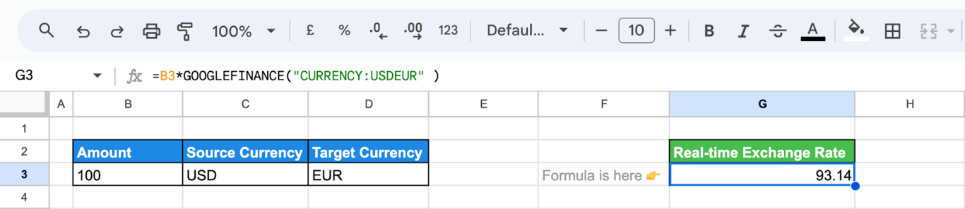
The result recalculates on its own as the rate changes. To show the rate itself, put the GOOGLEFINANCE part in its own cell and reference that cell in the multiplication. One rate cell is also easier to audit than the same function repeated in two hundred rows.

Convert a column with cell references

Typing the codes into the formula does not scale. Keep the source code in one column and the target code in another, and build the ticker from the cells:

=B3*GOOGLEFINANCE("CURRENCY:"&C3&D3)

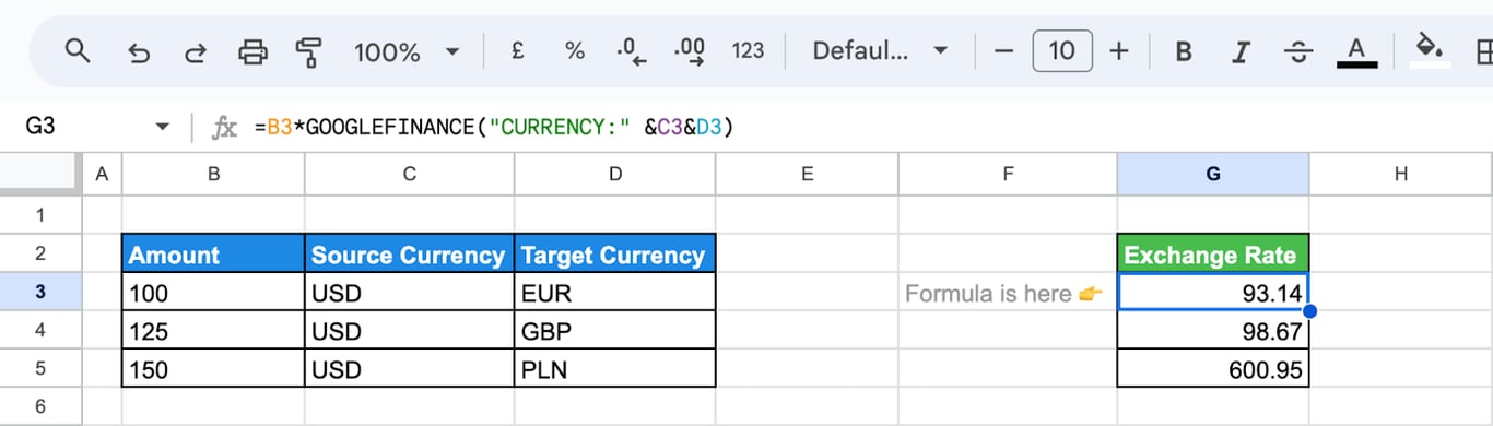
Here B3 holds the amount, C3 the source currency and D3 the target currency. Change a code in column D and the row recalculates for the new currency.

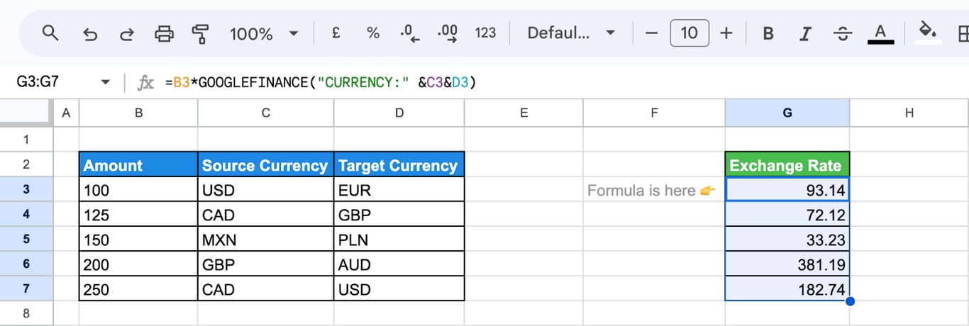
To apply the formula to the rows below, select the cell and drag the fill handle (the small square in its bottom right corner) down the column.

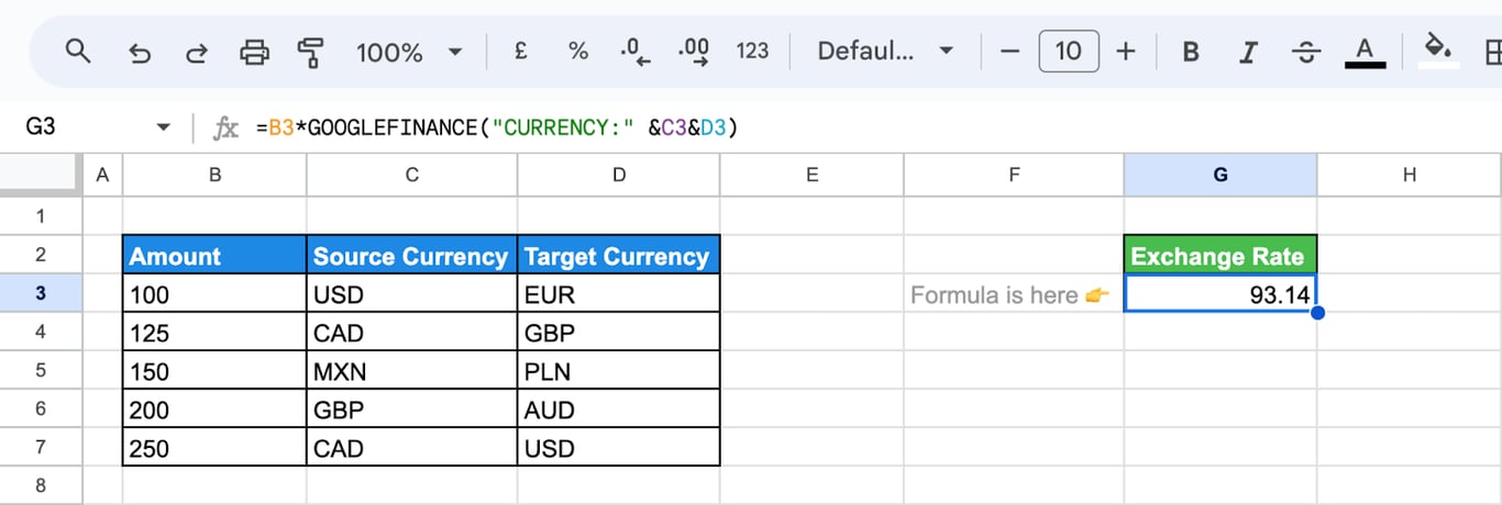
Each row now converts its own amount between its own pair of currencies.

Get a historical exchange rate

The rate on one day

Add the attribute and a date:

=GOOGLEFINANCE("CURRENCY:USDEUR", "price", DATE(2021,12,10))

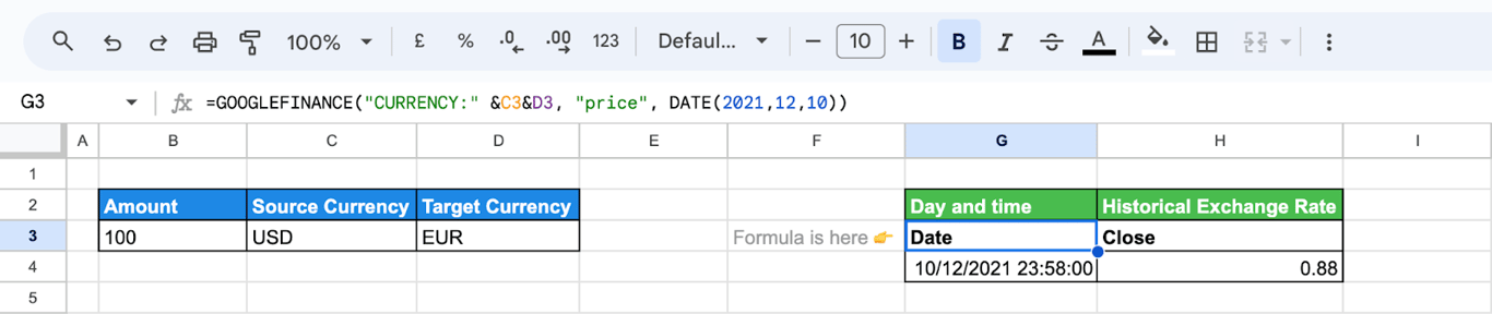
A historical request returns a small table, not a single number: a header row (Date, Close) and a row with the date and the closing rate. Leave the cells to the right and below empty, or the formula returns #REF!.

To get only the number, for example to multiply it by an amount, wrap the formula in INDEX and take the second row of the second column:

=INDEX(GOOGLEFINANCE("CURRENCY:USDEUR", "price", DATE(2021,12,10)), 2, 2)

The rates over a period

Give a start date and an end date, and an interval:

=GOOGLEFINANCE("CURRENCY:USDEUR", "price", DATE(2026,1,1), DATE(2026,1,31), "DAILY")

The result is one row per day. Use “WEEKLY” for one row per week. For a moving window, build the dates from TODAY: TODAY()-30 as the start date and TODAY() as the end date return the last 30 days and move forward by themselves.

What GOOGLEFINANCE rates are, and are not

Google states the limits on its GOOGLEFINANCE help page (checked October 2026):

• Rates can be delayed. Quotes “may be delayed up to 20 minutes”.
• They are for information, not for trading. The data is provided “as is” and solely for informational purposes.
• Historical data stays in the sheet. It cannot be downloaded or accessed through the Sheets API or Apps Script, so a script or an external tool reading the sheet will not get the historical values.

In practice this means GOOGLEFINANCE is right for a budget, a travel plan or a quick estimate. It is the wrong source for invoices, accounting or any report where the finance team already uses an official rate.

Common errors and how to fix them

#N/A

⚠️ Error: The formula returns #N/A.

✅ Solution: Check the ticker first: both codes must be valid, written together and in quotes, with “CURRENCY:” in front. If the ticker is built from cells, look for a stray space in the code cells. For a historical request, #N/A can also mean there is no data for that date; ask for a few days around it with num_days instead of a single date.

#REF!

⚠️ Error: A historical formula returns #REF!.

✅ Solution: The result table needs empty cells to the right and below. Clear them, or wrap the formula in INDEX to return a single value.

The codes change when the formula is copied

⚠️ Error: After dragging the formula down, some rows convert the wrong pair.

✅ Solution: If every row uses the same currency code stored in one cell, lock it with an absolute reference such as $D$1. Without the dollar signs, the reference moves down with each row.

The rate looks out of date

⚠️ Error: The rate in the sheet differs from the one you see elsewhere.

✅ Solution: A difference of a few minutes is expected, given the documented delay. Banks and payment providers also add their own margin, so their rate will not match a market rate. If you need the rate of a specific moment to stay fixed, copy the cell and paste it as a value (Edit → Paste special → Values only).

Related Google Sheets functions

Functions that are often used next to GOOGLEFINANCE, each with its own guide:

• VLOOKUP: Searches for a value in the first column of a range and returns a value from the same row.
• UNIQUE: Returns the distinct values of a range.
• QUERY: Filters, sorts and aggregates a range with an SQL-like syntax.
• MATCH: Returns the relative position of an item in a range.
• FILTER: Returns the rows of a range that meet your conditions.
• XLOOKUP: Searches a range for a match and returns the corresponding value from another range.
• IMPORTXML: Imports data from a web page or an XML feed using an XPath query.
• QUERY vs VLOOKUP: Compares the two functions and shows when each is the better choice.

One rate in a cell is not a rate the whole company uses

GOOGLEFINANCE answers “what is the rate right now” for one sheet. Reporting needs something else: the same daily rate applied to every row of ad spend or revenue, in every report, with a record of which rate was used on which day. A formula that recalculates in each copy of the sheet gives every copy a slightly different total.

The OWOX Data Marts extension for Google Sheets covers that half. A data analyst publishes a data mart (a table or an SQL query in your data warehouse) and makes it available for reports. In Sheets you open the extension, pick the data mart, tick the columns you want and run it. The rows land in a tab, ready for your formulas.

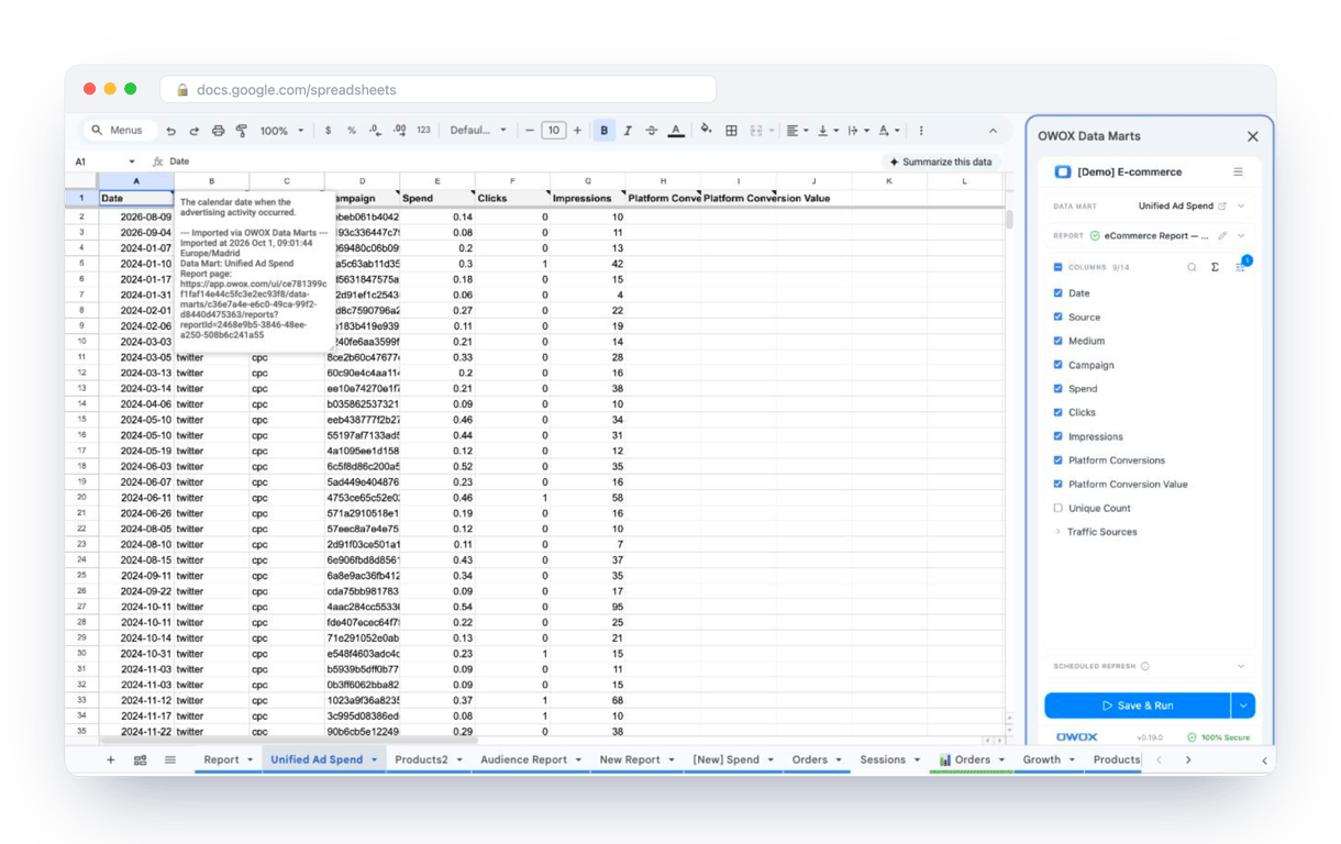
What changes for the person who maintains the sheet:

• Refresh replaces re-export. Refresh current report in the extension menu re-runs the same pull, and a scheduled refresh keeps the tab current without anyone touching it.
• The source is written on the sheet. The header cell of an imported tab carries a note with the data mart it came from, the time of the import and a link to the report.
• No SQL and no warehouse access needed. The analyst decides which data marts and columns are available. You choose from that list.

For currency reporting specifically, the rates can come from a data mart too: OWOX Data Marts loads daily rates from Open Exchange Rates into your warehouse, where the analyst joins them to spend, as described in Open Exchange Rates to Google Sheets. The extension does not write or change the analyst’s SQL, and GOOGLEFINANCE stays the quickest way to check a rate. The extension comes with the OWOX Cloud plans of OWOX Data Marts; spreadsheet reporting describes both ways data reaches a sheet.

Google Sheets TipsHow to search in Google Sheets: Ctrl+F and the SEARCH functionOctober 2, 2026→Google Sheets TipsQUERY with UNIQUE in Google Sheets: return distinct rowsOctober 2, 2026→Google Sheets TipsFILTER function in Google Sheets: formula and examplesOctober 2, 2026→

See all articles →