How to Sort Data in Google Sheets: A Complete Guide

Data, when organized well, tells a compelling story. Sorting data in Google Sheets is more than just arranging rows and columns- it’s a powerful way to uncover trends, streamline workflows, and make smarter decisions. 

Whether you’re analyzing sales figures, managing inventory, or tracking campaign performance, mastering sorting techniques can save time and eliminate errors, giving you more control over your data.

Imagine quickly alphabetizing customer lists, sorting by highest sales, or organizing project timelines by deadlines - all with a few clicks. This guide will take you from basic sorting methods to advanced automation techniques, ensuring your data stays organized and actionable. Let’s explore how to make Google Sheets your go-to tool for efficient data management.

Benefits of Sorting Data in Google Sheets

Sorting data in Google Sheets is an essential skill for keeping your spreadsheets organized and easy to analyze. 

Whether you're managing customer lists, tracking sales, or organizing campaign data, sorting ensures your information is clear, structured, and ready for action.

Here are the key benefits of sorting data in Google Sheets:

• Improves Data Accessibility: Sorting data allows you to quickly find and access specific information, making it easier to analyze, report, and make decisions.
• Enhances Data Accuracy: Proper sorting ensures data is organized correctly, reducing the risk of errors when interpreting or processing information.
• Facilitates Trend Analysis: Sorting helps highlight patterns, trends, and outliers within your dataset, enabling better insights for decision-making.
• Boosts Efficiency: By sorting your data, you reduce the time spent on manual searches and enhance your ability to work faster and more effectively with large datasets.
• Improves Data Presentation: Well-sorted data is more visually appealing and easier to understand, which is essential for reporting and sharing with stakeholders.

Basic Sorting Techniques in Google Sheets

Basic sorting techniques in Google Sheets is key to organizing your data effectively. Whether you need to arrange information alphabetically, by date, or by numerical value, these methods provide a strong foundation for managing datasets.

Download Your Ultimate Sorting Data Template Now!

All the functions and examples from this guide are prepped and ready for you. Simply download, click, and dive into Sorting Data in Google Sheets. Start practicing instantly!

Get your FREE template now!

Sorting Data Alphabetically

Sorting data alphabetically in Google Sheets is a fundamental technique for organizing text-based data. Google Sheets provides two primary options: sorting the entire sheet or sorting a specific range. Each method caters to different organizational needs while preserving the integrity of your data.

Types of Sorting:

1. Sort Sheet: Sorts all rows in the sheet based on a specific column, keeping related information in each row intact. Ideal for organizing entire datasets comprehensively.
2. Sort Range: Sorts only the selected range of cells, leaving other parts of the sheet unaffected. Useful for managing multiple tables or isolated datasets within the same sheet.

Example of Sort Sheet:

In this example, we'll alphabetically sort the entire dataset by the Customer Name column, ensuring all information in each row stays intact.

Steps to Sort the Sheet:

• Enter the dataset above into a column. Place Customer Name as the header in the cell.

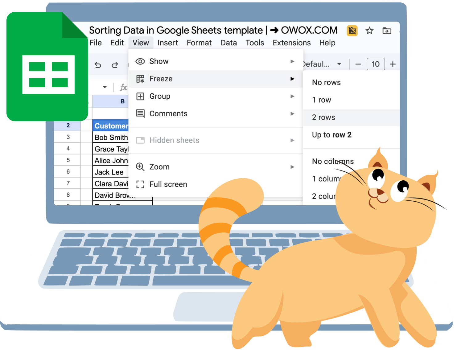
• Go to the View menu.
• Hover over Freeze and select 2 rows to ensure the header remains unaffected during sorting.

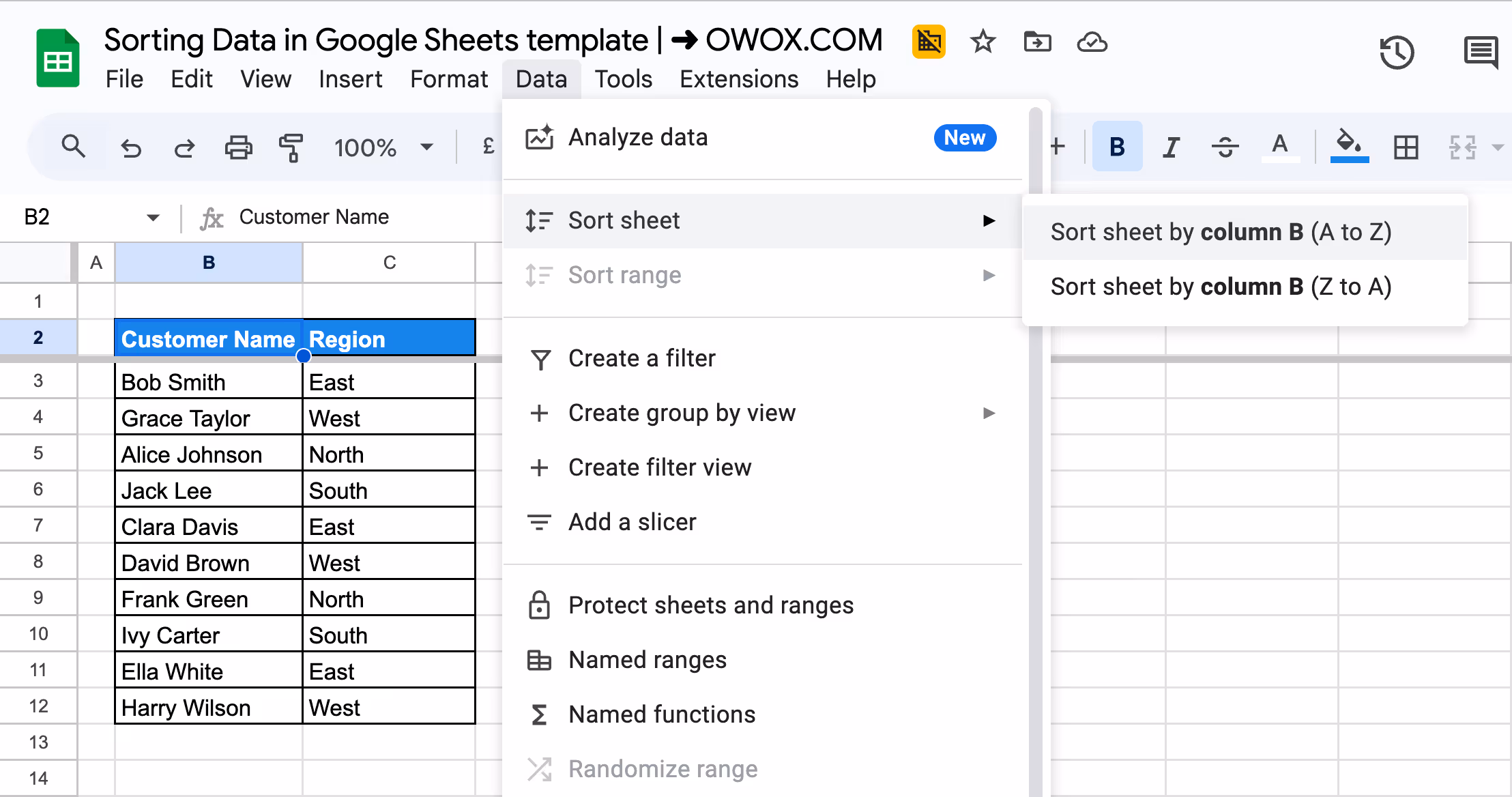
• Click on any cell within the Customer Name column, such as B3.

• Go to the top menu and click on Data.
• Choose Sort Sheet by Column B (A-Z) to sort in ascending alphabetical order.

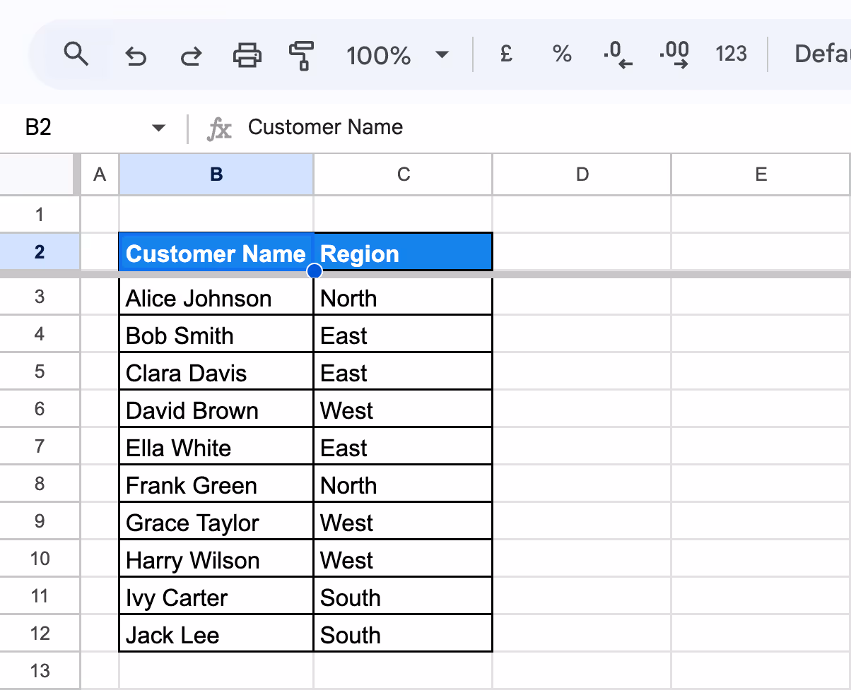
• For ascending order (A-Z), the first name in the list will be Alice Johnson, and the last name will be Jack Lee.

The entire dataset will be sorted alphabetically by customer names, keeping all rows intact.

Sort Range Example:

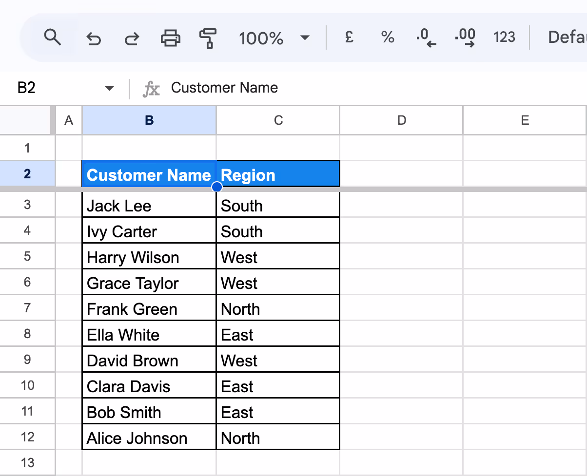
Now, let's sort only a specific range of data (e.g., the Customer Name and Region columns).

1. Place Customer Name in column B and Region in column C.

2. Highlight the range of cells you want to sort:

• Click and drag to select from B15 to C24 (do not include the header row).
• The selected range should now be highlighted.

3.  Go to the top menu bar and click on Data.
4.  From the drop-down menu, select Sort range.
5.  Access Advanced Sorting Options

6.  A dialog box titled Sort range options will appear.

In the dialog box:

• From the Sort by drop-down, select Column B (Customer Name).
• Choose A → Z for ascending order.

7. Click Sort to apply the sorting.

Only the selected range will be sorted alphabetically by customer names, while the rest of the sheet remains unchanged.

Sort Data with a Header Row

When your dataset includes a header row, freezing it ensures that the headers are excluded from sorting. If the header row isn't frozen, it may get sorted along with the data, leading to confusion. Freezing the header row keeps column labels intact for clarity.

Example of Sorting Data with a Header Row:

In this example, we’ll sort the dataset by Customer Name alphabetically while ensuring the header row remains fixed.

• Enter Customer Name in column B and Region in column C.
• Freeze the Header Row‍
• Locate the gray horizontal line in the top-left corner of the sheet (above row numbers).
• Drag it down below the header row, between rows 1 and 2. This locks the header row in place.

• Click on any cell in the Customer Name column, such as B3, to sort by customer names.
• Navigate to Data > Sort Sheet by Column A (A-Z) to sort customer names alphabetically.

• Here is how your data will look like after sorting.

• Alternatively, select Data > Sort Sheet by Column A (Z-A) to sort names in reverse alphabetical order.

Sorting Data by Date

Sorting data by date helps you arrange records chronologically, making tracking events, analyzing timelines, or managing schedules easier. 

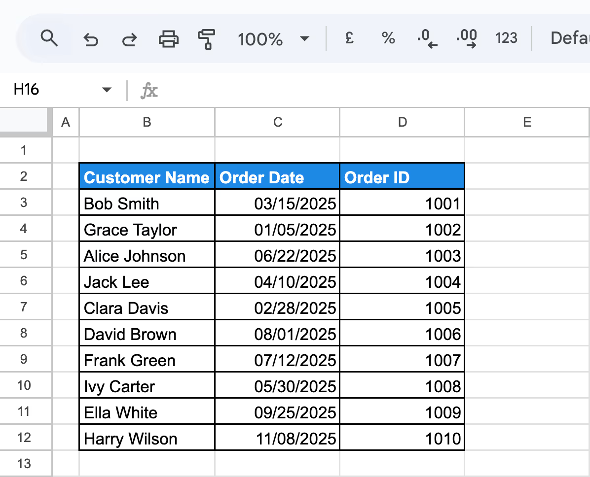
Example: Sorting the Dataset by Order Date

In this example, we’ll sort the dataset by the Order Date column in ascending order, ensuring the orders are arranged chronologically. This is particularly useful for tracking sales progression over time.

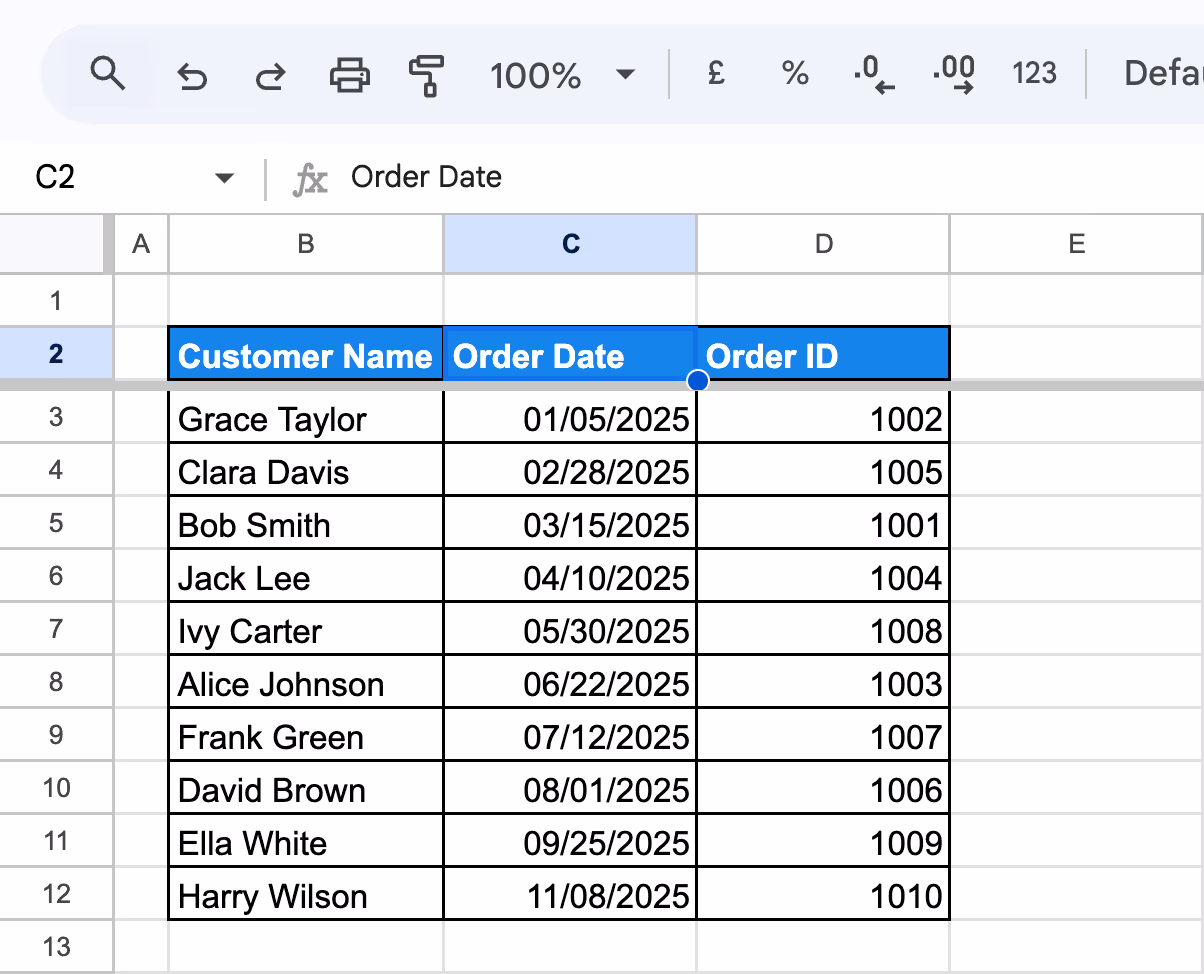
• Click on any cell in the Order Date column, such as C3.

• Freeze the Header Row (Optional but Recommended)

• Navigate to Data > Sort Sheet by Column C (A-Z) to sort dates in ascending order (oldest to newest).

• Alternatively, choose Sort Sheet by Column C (Z-A) to sort dates in descending order (newest to oldest).

Sorting Data by Numerical Value

Sorting data by numerical value in Google Sheets helps you organize datasets based on quantities, prices, or any numerical metric. This technique is ideal for identifying trends, comparing values, or prioritizing key data points effectively.

Sort Data from Lowest to Highest

Sorting data from lowest to highest organizes numerical values in ascending order, helping you identify the smallest values first.

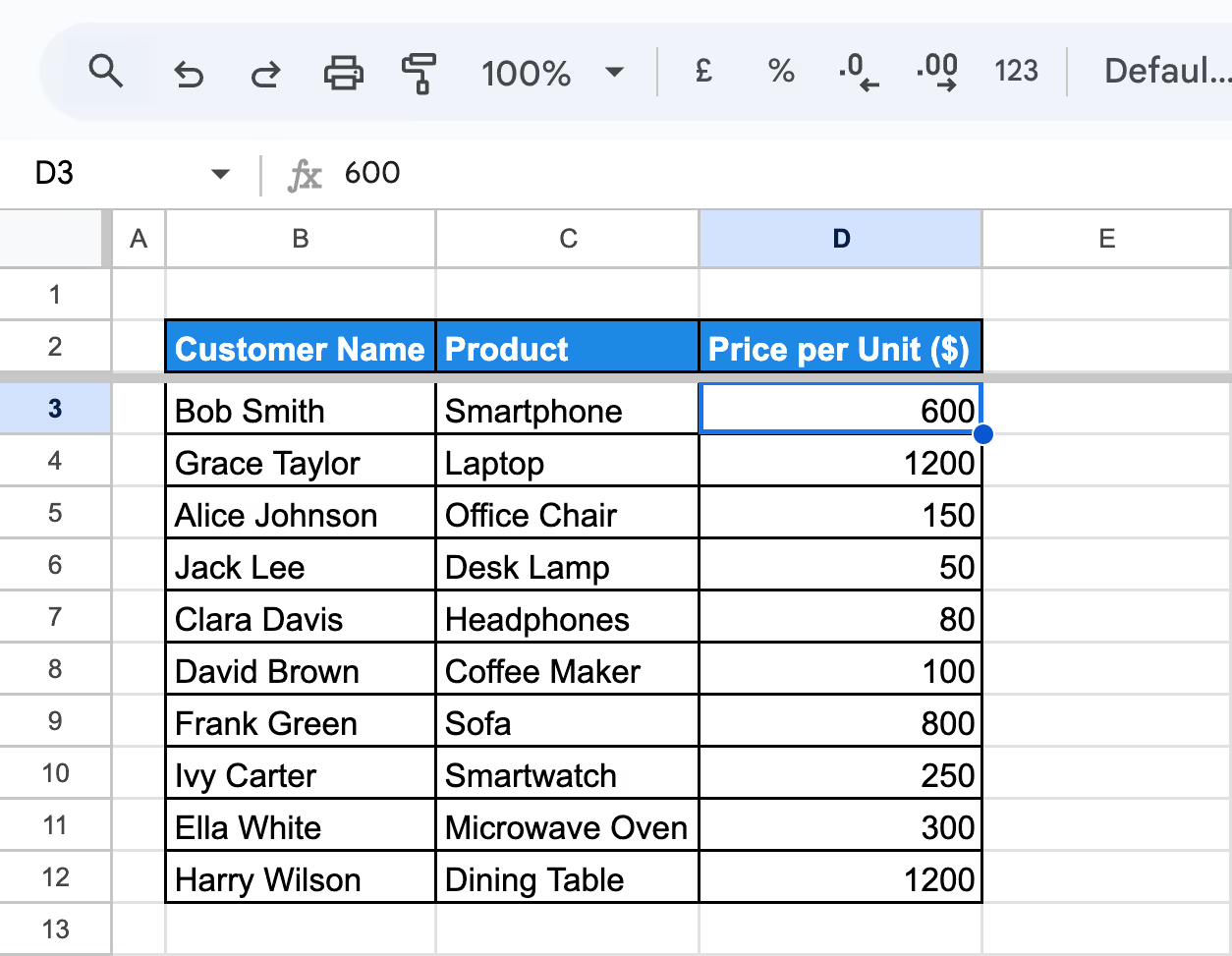
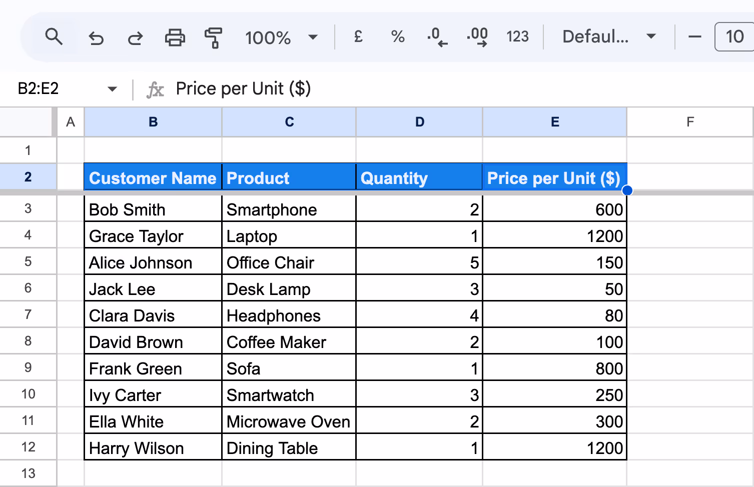
Example: Sorting by Price per Unit ($)

In this example, we’ll sort the dataset by the Price per Unit ($) column to display the products from the lowest price to the highest.

• Freeze the Header Row (as shown in the previous examples)
• Click on any cell in the Price per Unit ($) column, such as D3.

•  Select Sort Sheet by Column D (A-Z) to sort the prices in ascending order.

• The dataset will now be sorted, displaying products starting from the lowest price to the highest.

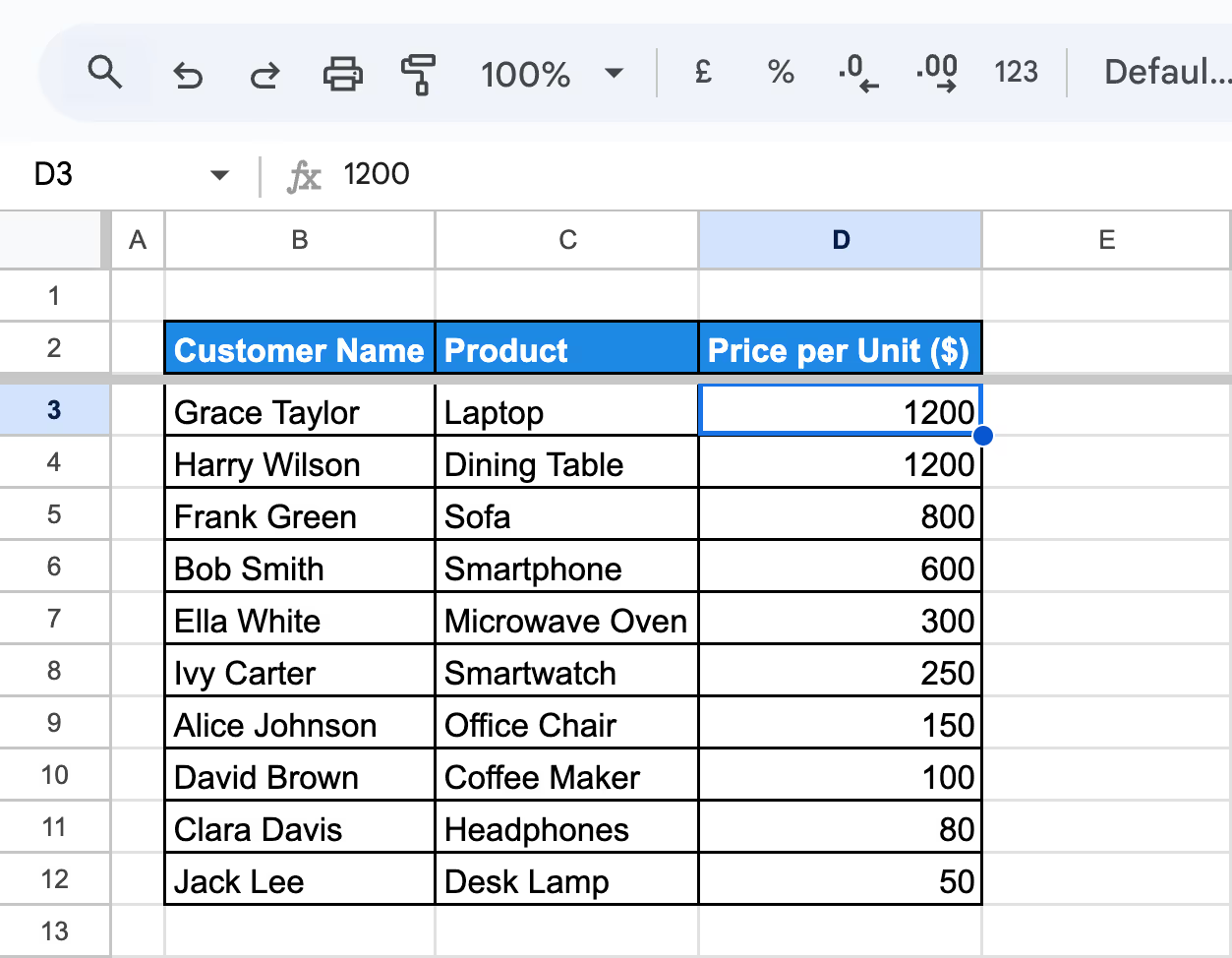
Sort Data from Highest to Lowest

Sorting data from highest to lowest organizes numerical values in descending order, making it easy to identify the largest values first.

Example: Sorting by Price per Unit ($)

In this example, we’ll sort the dataset by the Price per Unit ($) column to display products from the highest price to the lowest.

• Click on any cell in the Price per Unit ($) column, such as D3.

• Select Sort Sheet by Column C (Z-A) to sort the prices in descending order.

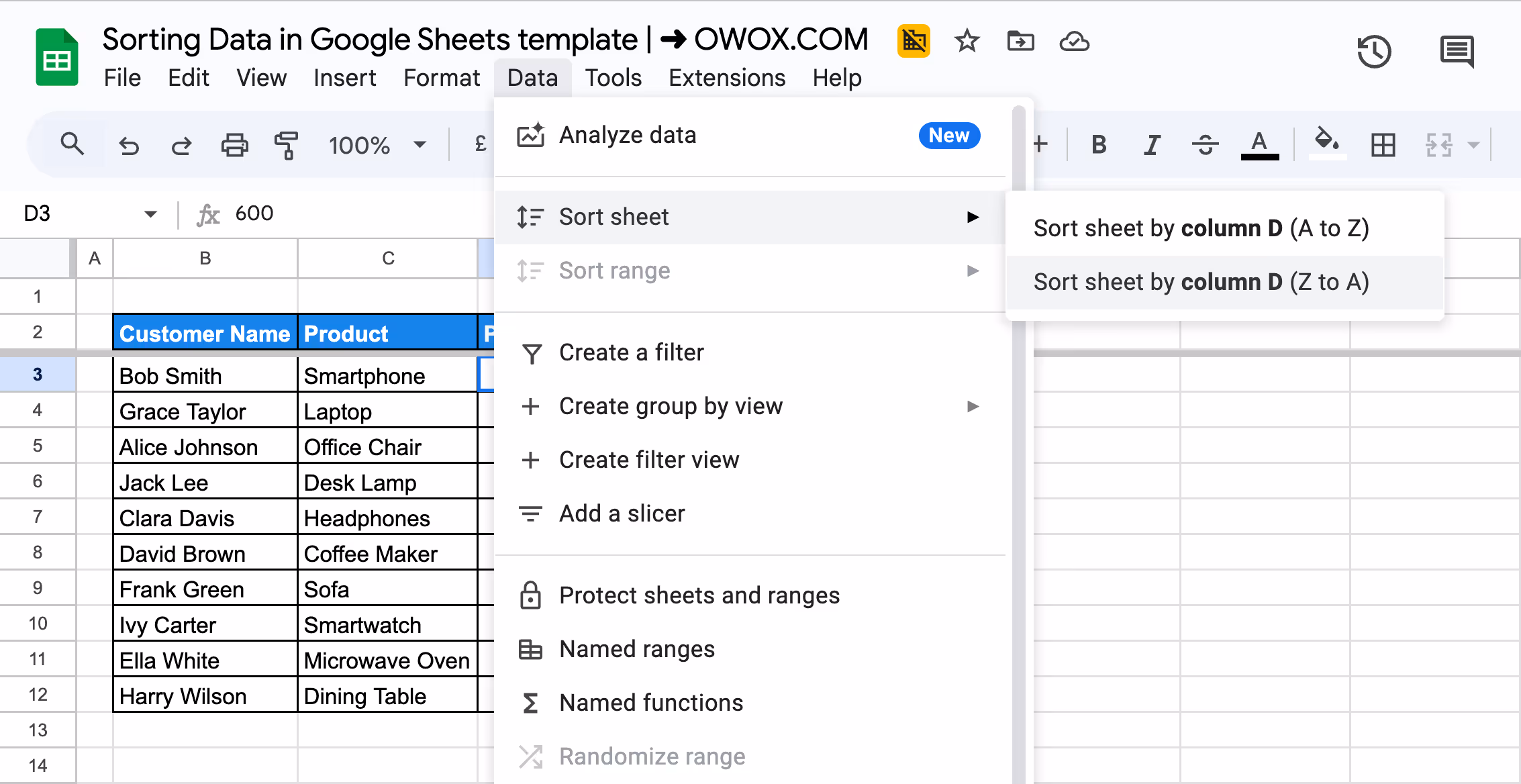
• The dataset will now be sorted, displaying products starting from the highest price to the lowest.

Advanced Sorting Techniques in Google Sheets

Advanced sorting techniques in Google Sheets allow you to go beyond basic sorting. These methods enable you to organize data more effectively, uncover deeper insights, and tailor sorting to complex datasets with ease.

Sorting Values with a Filter

Sorting and filtering are often confused, but they serve different purposes. Sorting arranges data in ascending or descending order, while filtering hides unnecessary data to focus only on specific values.

Example 1: Filtering by Region

In this example, we will filter the dataset to show only rows with the East Region.

• Click on Data > Create a Filter to activate filters.

• Click the filter icon in the Region column header.
• Select Filter by values and uncheck all boxes except East.

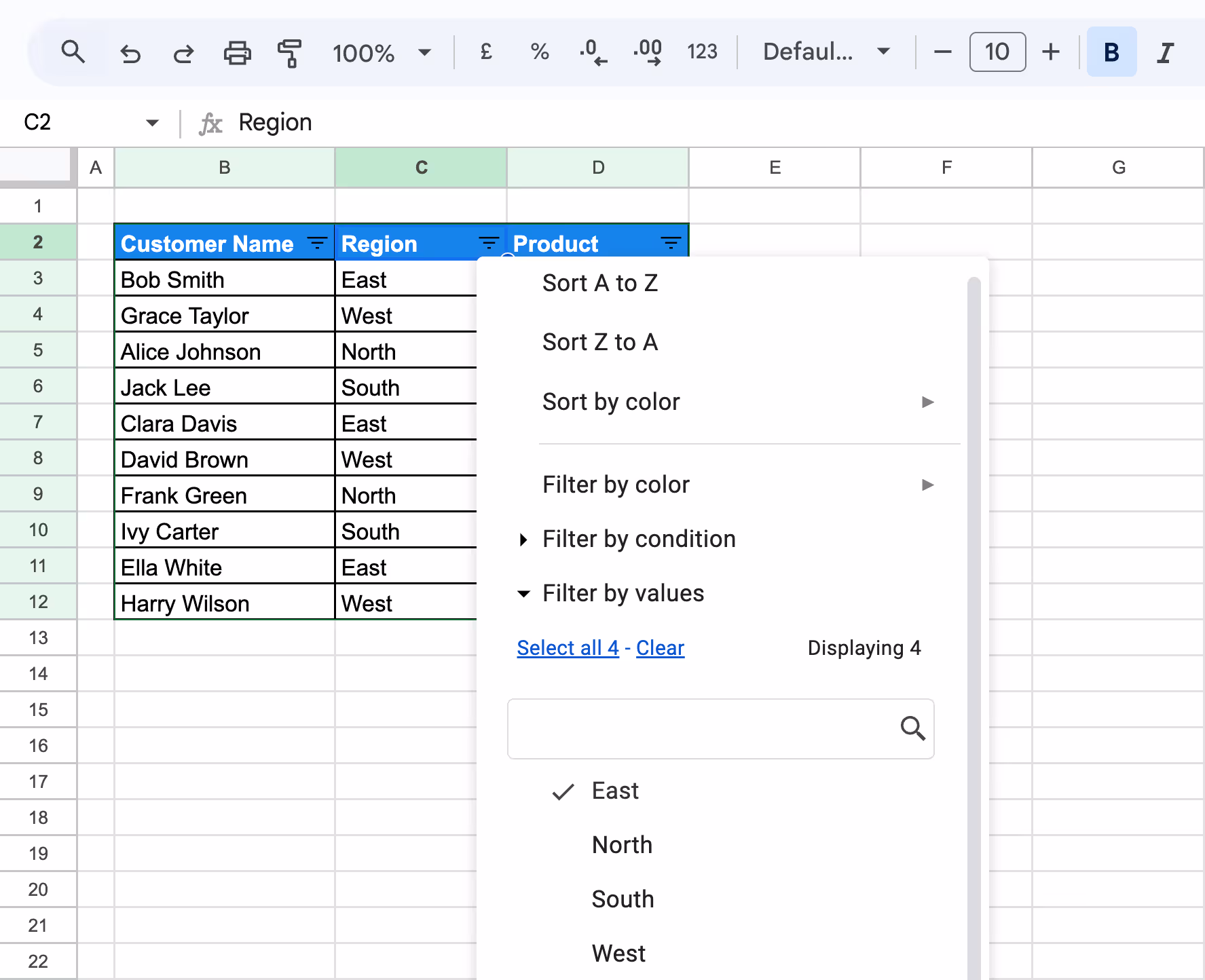
• Click OK to apply the filter.

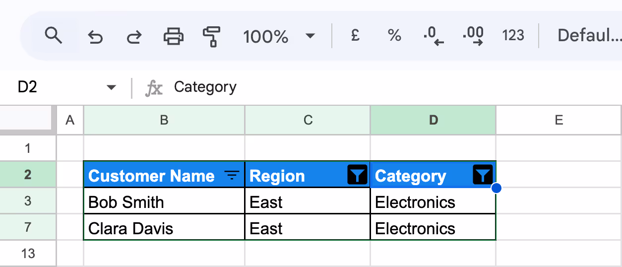
Example 2: Cumulative Filtering for East Region and Product

Now, we’ll replace the “Product” column with the “Category” column and filter the dataset to show only records from the East region with categories related to Electronics.

• Follow the same steps with this data set as in Example 1.

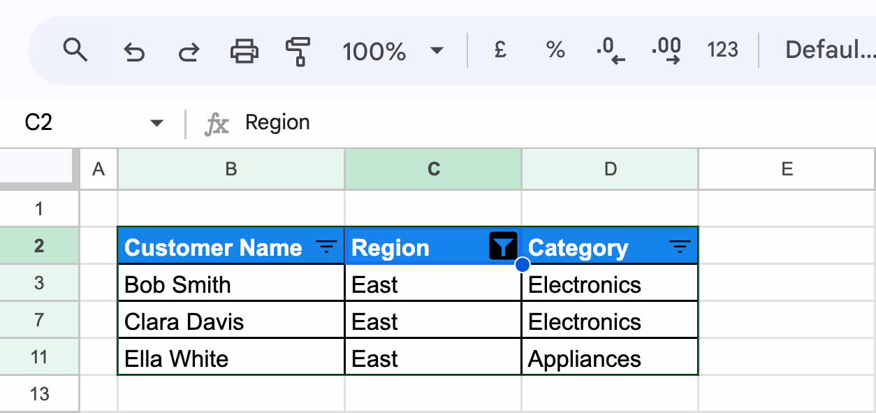
• Click the filter icon in the Category column header.
• Select Filter by values and uncheck all boxes except Electronics.

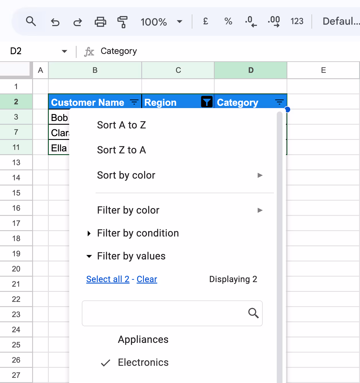
• Click OK to apply the additional filter.
• The dataset will now display records from the East region with Electronics products only.

‍

💡 Master the FILTER function in Google Sheets to refine and analyze your data effortlessly. Check out this comprehensive guide for step-by-step instructions and examples: Google Sheets FILTER Function. 

Dive deeper with this read

The Ultimate Guide to Using the FILTER Function in Google Sheets

Sorting Values with a Filter View

A Filter View in Google Sheets allows you to sort and filter data temporarily without affecting the original dataset. This feature is ideal for collaborative projects where multiple users must analyze data differently without interfering with one another’s views.

Example:

In this example, we’ll alphabetically sort the dataset by the Product column using a Filter View. This allows for temporary sorting that doesn’t impact the original structure.

Step 1: Set up the dataset.

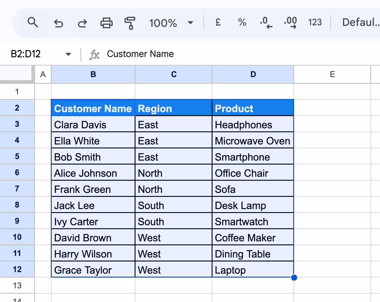
Step 2: Select the entire dataset or columns you want to work with.

Step 3: Go to Data > Create Filter View.

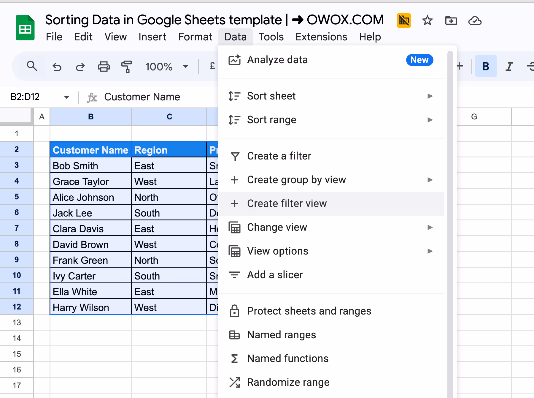
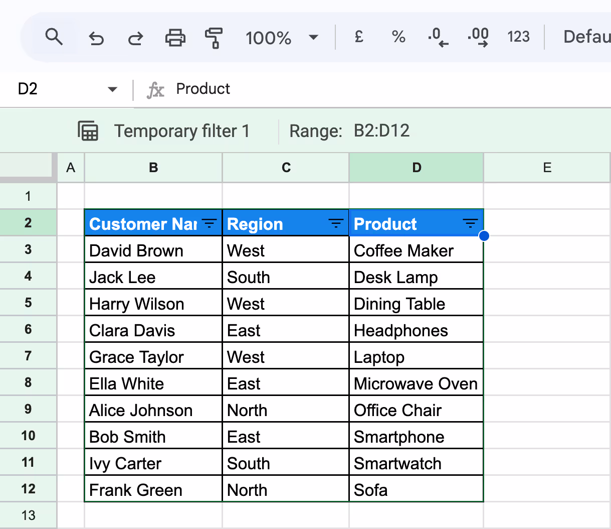
• At this point, you should see a temporary view.

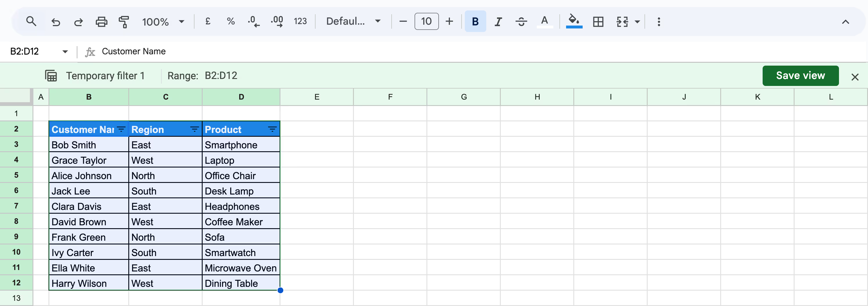
Step 4: In the drop-down menu, choose Sort A to Z to arrange the products alphabetically (in ascending order).

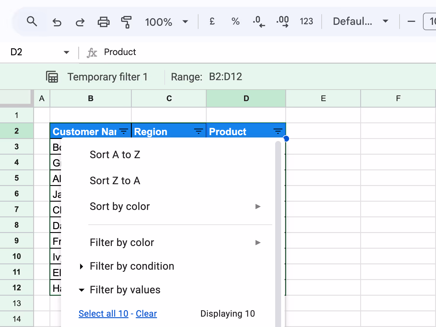
The data in the Product column will now appear sorted within the Filter View without altering the original dataset outside of this view.

Sorting Data by Multiple Columns

Sorting data by multiple columns in Google Sheets allows you to organize your dataset with layered criteria. This method benefits large datasets where sorting by a single column may not provide sufficient clarity.

Example: Sorting by Region and Product

In this example, we’ll sort the dataset by the Region column alphabetically and then by the Product column alphabetically within each region.

Step 1: Set up the dataset.

Step 2: Select the range of cells to include headers.

Step 3: Navigate to Data > Sort range > Advanced range sorting options.

Step 4:  Check the box for Data that has the header row to exclude the header from the sorting process.

Step 5: In the Sort by dropdown, select Region.

Step 6: Add a secondary sorting column, and click Add another sort column. In the dropdown, select Product.

Step 7: Apply the Sorting

The dataset will now be grouped by region and sorted alphabetically by product within each region.

Sorting Data by Color

Sorting data by color in Google Sheets allows you to group rows based on fill or text color, making it easier to highlight specific categories or prioritize tasks visually.

Example: Sorting Rows by Fill Color

In this example, we’ll sort the dataset based on the fill color used in the Region column, grouping rows with the same color-coded regions together for easier analysis.

Step 1: Set Up the Dataset

Step 2: Click Data > Create a Filter to activate filters for the dataset.

Step 3: Click the filter icon in the Region column header.

Step 4: Hover over Sort by color and choose Fill color.

Step 5: Choose Green (🟩) to group rows from the East region at the top.

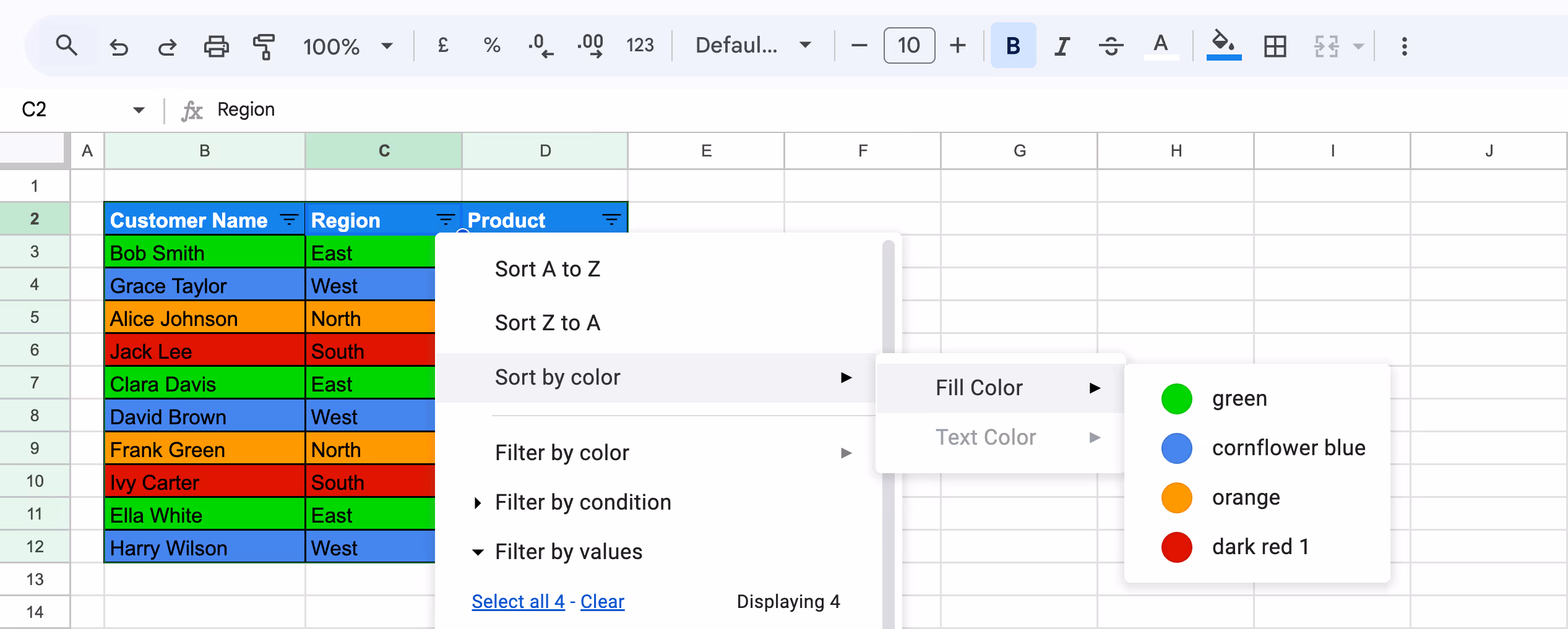
Step 6:  Repeat the sorting process for other colors (e.g., blue for West, orange for North, and red for South) to group rows accordingly.

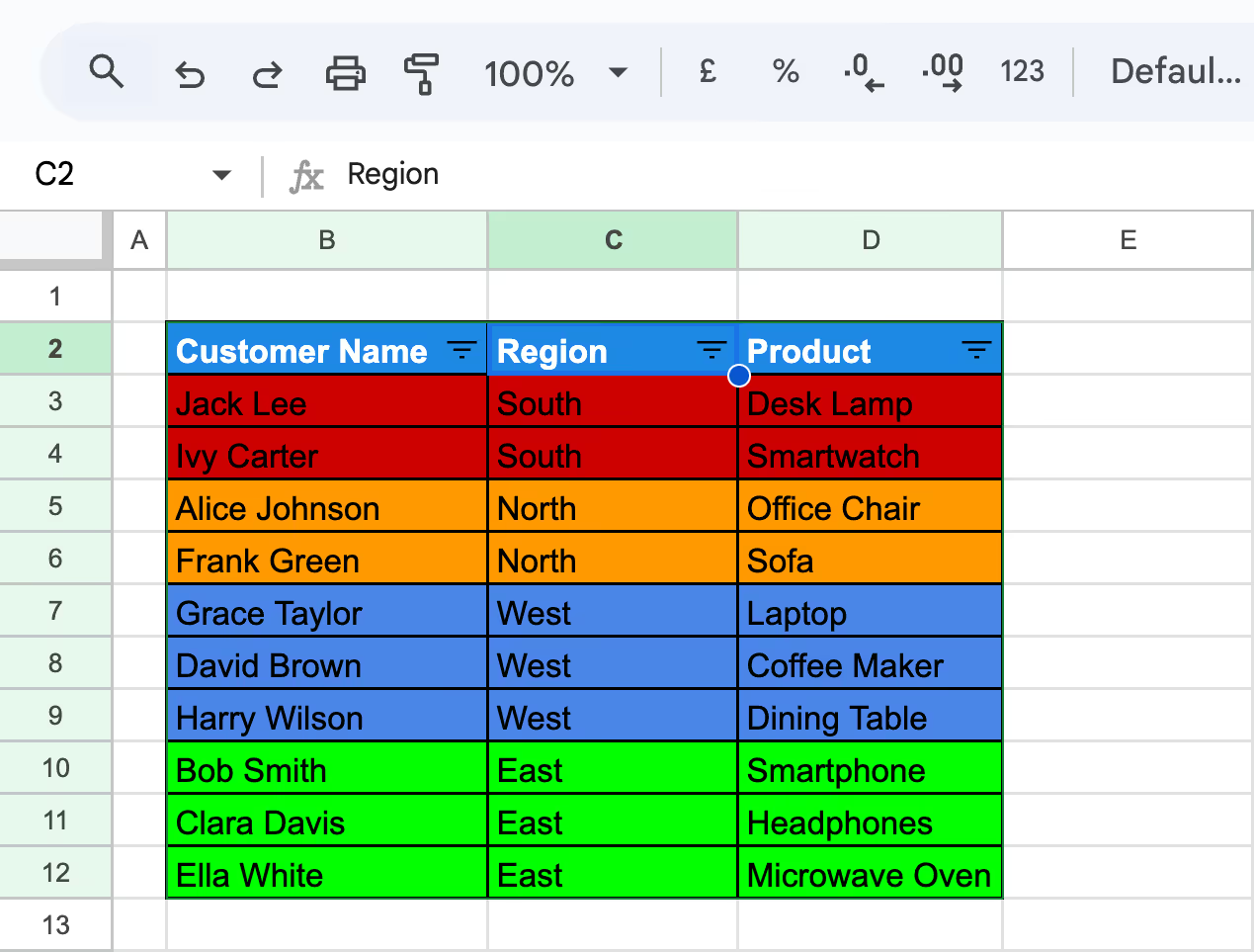
The dataset will now be sorted and grouped by fill color in the Region column.

Efficient Sorting and Function Automation Techniques in Google Sheets

Sorting and automation techniques in Google Sheets streamline data organization and enhance productivity. Combining sorting with powerful functions allows you to automate repetitive tasks, maintain dynamic datasets, and analyze data effortlessly.

Handling ARRAYFORMULA Calculations After Sorting

ARRAYFORMULA calculations can be disrupted if they are placed within the dataset itself and the data is later sorted. Sorting changes the relative cell references, leading to misaligned or broken results. 

To avoid this, always place ARRAYFORMULA calculations in the header section, ensuring the formula remains unaffected by sorting.

Example:

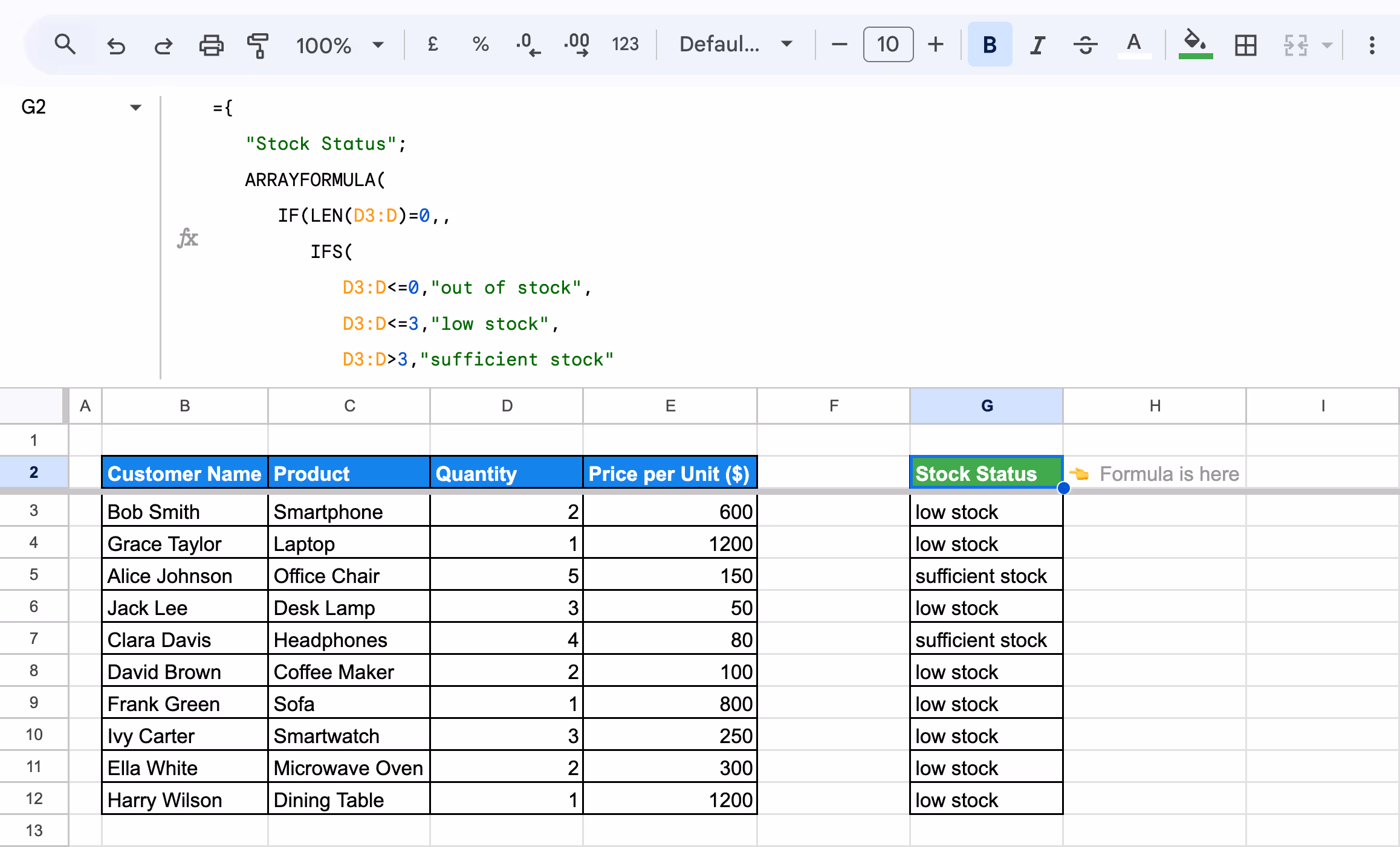
In this example, we’ll calculate the stock status for products using the Quantity column (located in column D) and ensure the ARRAYFORMULA remains intact even after sorting.

Use this formula in Column G2:

={
  "Stock Status";
  ARRAYFORMULA(
      IF(LEN(D3:D)=0,,
        IFS(
            D3:D<=0,"out of stock",
            D3:D<=3,"low stock",
            D3:D>3,"sufficient stock"
        )
      )
  )
}

Here:

• "Stock Status": Adds a dynamic header for the calculated column.
• ARRAYFORMULA: Extends the formula to apply to all rows in the specified range.
• LEN(D2:D)=0: Ignores empty rows in the column.
• IFS: Assigns stock status based on the following conditions:
• <=0: "Out of stock" for zero or negative values.
• <=3: "Low stock" for quantities between 1 and 3.
• >3: "Sufficient stock" for quantities above 3.

Next, Sort the data by any column (e.g., Customer Name or Product) using Data > Sort Sheet.

Placing ARRAYFORMULA calculations in the header section ensures they remain unaffected by sorting.

💡 Dive deeper into the power of ARRAYFORMULA and how it can simplify your calculations in Google Sheets. Check out our comprehensive guide here: Mastering ARRAYFORMULA in Google Sheets. 

Dive deeper with this read

Mastering ARRAYFORMULA in Google Sheets: A Complete Guide

Using SUMIF for Stable Calculations After Sorting

Sorting datasets in Google Sheets can disrupt calculations if static cell references are used, as the references will no longer point to the intended data. To avoid this, dynamic functions like SUMIF ensure calculations remain stable by using specific criteria rather than fixed cell references.

Example: Summing the Total Number of Furniture Products

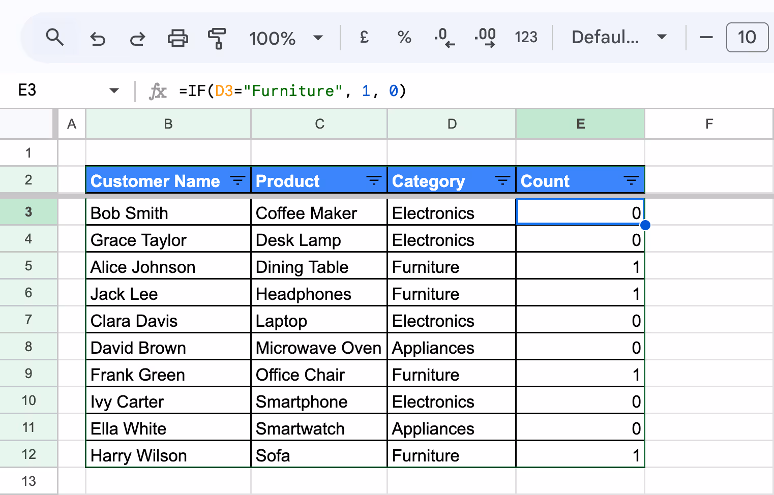
In this example, we will calculate the total count of Furniture items using the SUMIF function. To ensure the calculation is unaffected by sorting, a helper column will be used to assign values dynamically based on the condition.

1. Create a new column named Count next to your dataset.
2. In cell E3, enter the following formula:

=IF(D3="Furniture", 1, 0)

3. Drag the formula down to apply it to all rows.

4. Use the following formula to calculate the total count of Furniture items:

=SUMIF(D3:D, "Furniture", E3:E)

Here:

• Helper Column: Dynamically assigns 1 for rows where the Category is "Furniture" and 0 otherwise.
• SUMIF: Sums up the values in the Count column (E2:E) where the condition "Furniture" is met in the Category column (D2:D).

5. Sort the dataset by any column (e.g., Customer Name or Product).

By adding a helper column and using SUMIF, you can calculate totals dynamically based on specific criteria, ensuring stable calculations even after sorting the dataset.

Using the QUERY Function to Sort with Blank Rows at the Top

In Google Sheets, sorting a dataset typically moves blank rows to the bottom, regardless of whether the sort order is ascending or descending. However, with the QUERY function, you can modify the sorting behavior to keep blank rows at the top of your dataset.

Example: Sorting with Blank Rows at the Top

In this example, we’ll use the QUERY function to sort a dataset by the Products column while ensuring blank rows remain at the top.

Use the following formula in a blank cell, such as G3:

=QUERY('Using the QUERY Function to Sort with Blank Rows at the Top'!B3:D10, "select * order by C")

Here:

• 'Using the QUERY Function to Sort with Blank Rows at the Top': Refers to the sheet's name containing your dataset. The name is enclosed in single quotes due to spaces.
• B3:D10: Specifies the data range, starting from row 3 to row 10, including blank rows.
• select *: Selects all columns (Customer Name, Product, and Region).
• order by C: Sorts the dataset by the Product column (C) in ascending order.

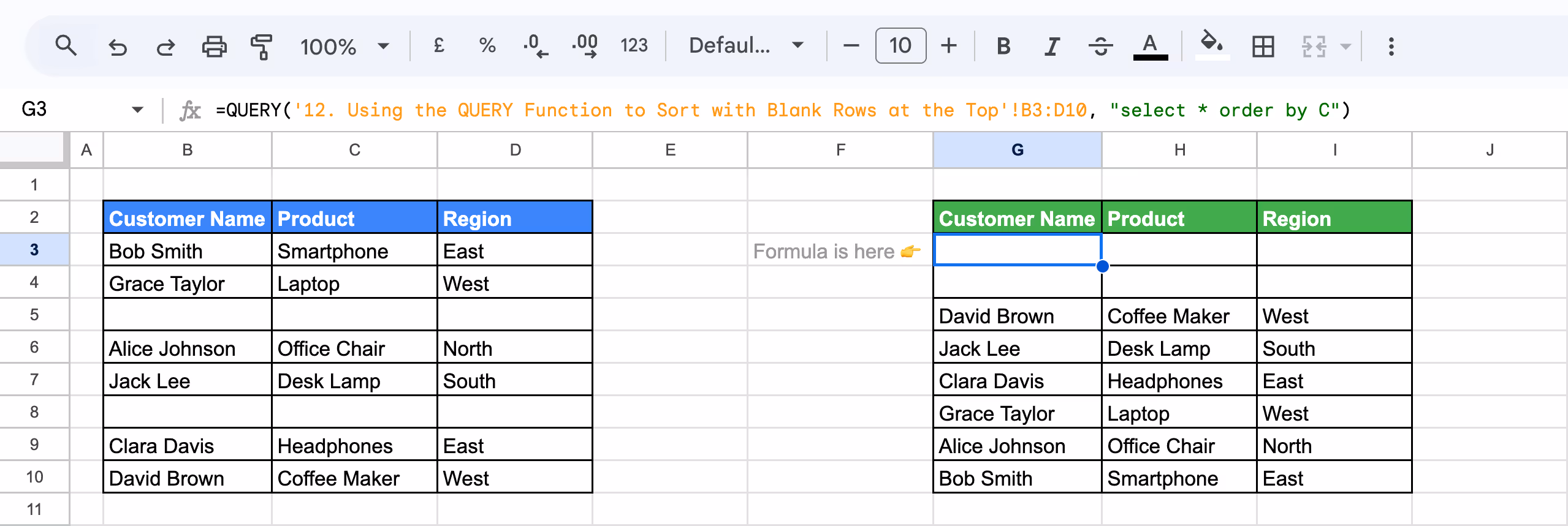
Using the QUERY function, you can dynamically sort data by any column while keeping blank rows at the top. 

💡 Learn how to unleash the full potential of the QUERY function in Google Sheets. Check out this in-depth guide: Mastering the QUERY Function in Google Sheets. 

Dive deeper with this read

Google Sheets Query Function: Tips for Efficient Data Management

Sorting Data in Google Sheets Using the SORT Function

The SORT function in Google Sheets offers a simple and efficient way to organize data based on specific columns dynamically. Unlike manual sorting, it updates automatically when the data changes, making it ideal for maintaining organized and up-to-date datasets without repeated effort.

Sorting Data Dynamically Using SORT Function in Google Sheets

The SORT function in Google Sheets allows you to arrange your data by specific columns dynamically. It eliminates manual sorting, automatically updating as your dataset changes, making it perfect for real-time analysis and streamlined workflows.

Example: 

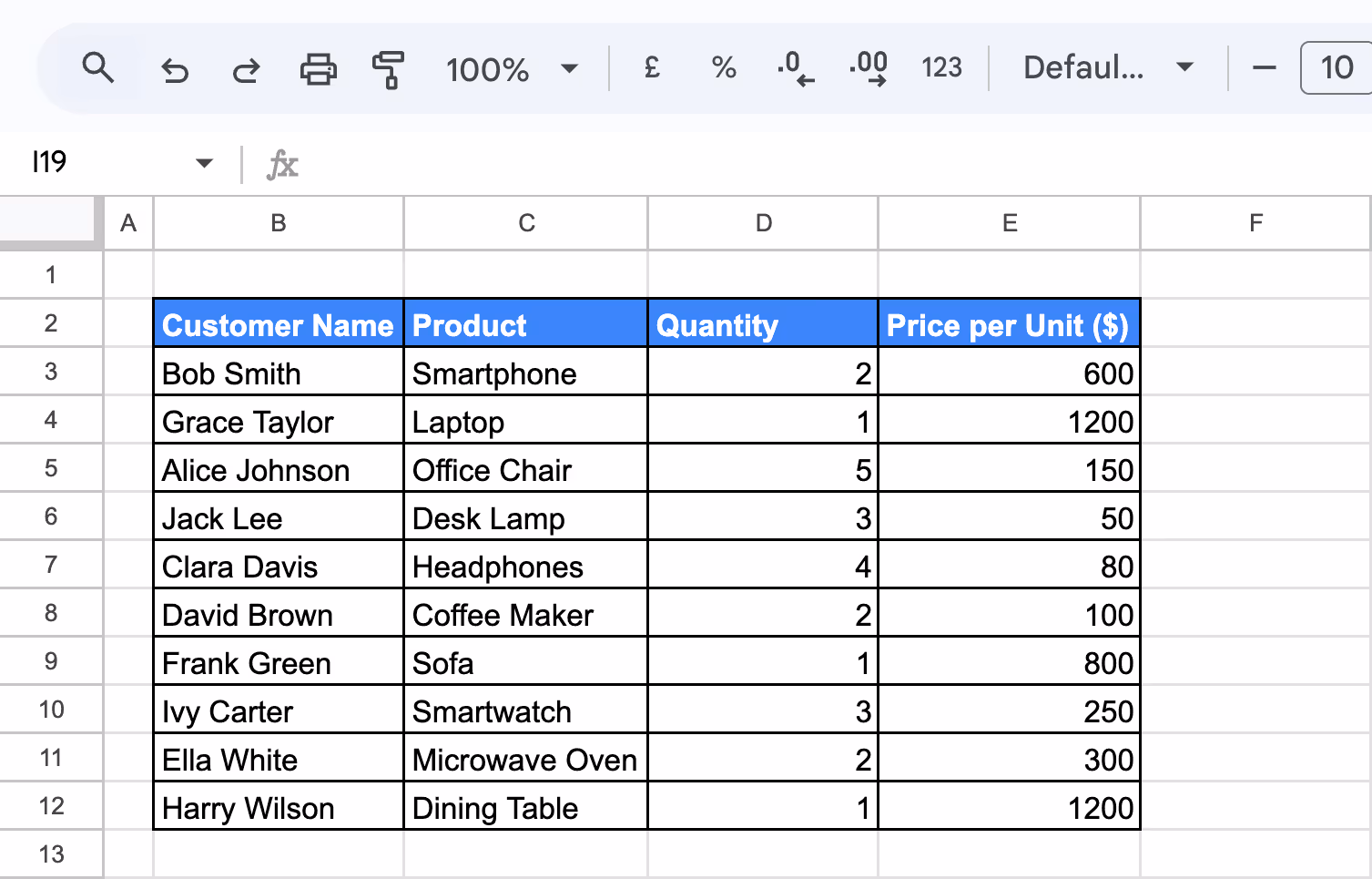
In this example, we’ll auto-sort the dataset by the Price per Unit ($) column in descending order, automatically sorting any newly added rows. The original sheet contains the dataset "Sorting Data Dynamically using SORT function in Google Sheets.”

Steps to Use the SORT Function Dynamically:

• Create a New Sheet
  
  • Add a new sheet for the sorted data.

• Enter the Formula

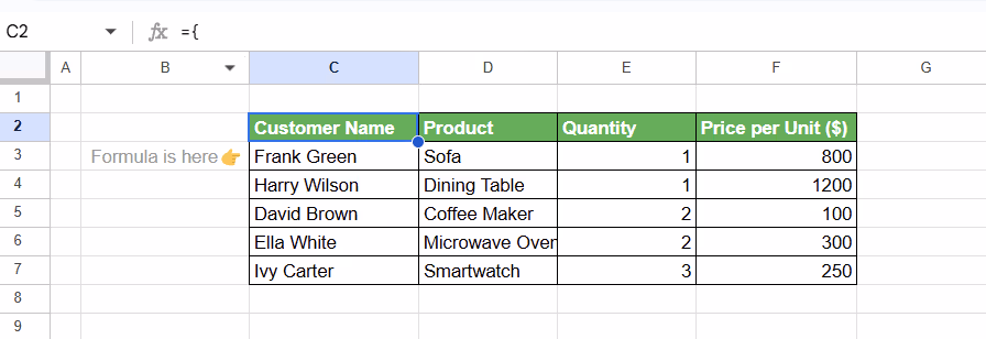
In cell B2 of the new sheet, enter the following formula:

={
  "Customer Name", "Product", "Quantity", "Price per Unit ($)";
  SORT('Sorting Data Dynamically using SORT function in Google Sheets'!B3:E, 'Sorting Data Dynamically using SORT function in Google Sheets'!E3:E, FALSE)
}

Here:

• "Customer Name", "Product", "Quantity", "Price per Unit ($)": Creates headers dynamically in the new sheet.
• SORT: Sorts the data based on specified criteria:
• B3:E: The data range from the original sheet (excluding headers).
• E3:E: The column to sort by (Price per Unit ($)).
• FALSE: Sorts the data in descending order.

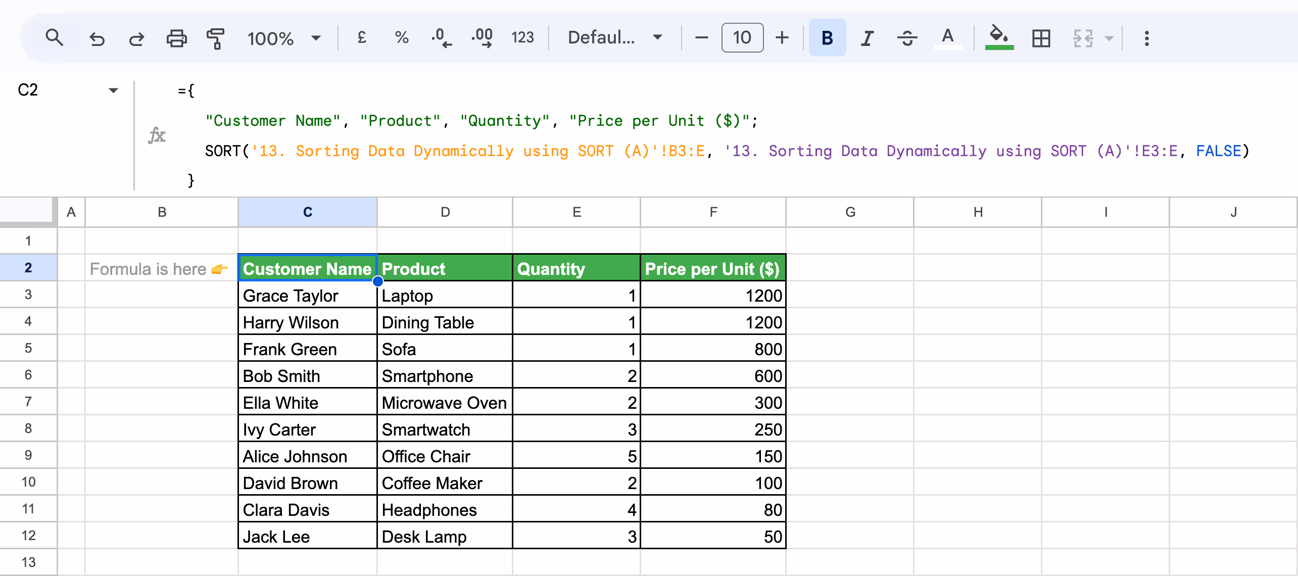
The formula dynamically sorts the dataset in descending order of Price per Unit ($).

Automatically Sorting Data Using SORT into Separate Sheets

The SORT function in Google Sheets helps organize data dynamically and split and sort data into different sheets. By specifying the data range and sort criteria for each sheet, you can manage subsets of your data more effectively.

Example:

In this example, we’ll demonstrate how to split a dataset into two chunks and dynamically sort them into separate sheets using the SORT function. 

We will be using the same dataset already present in the sheet named  "Sorting Data Dynamically using SORT function in Google Sheets.”

The first sheet will sort the data by Price per Unit ($) in descending order, while the second sheet will sort by Quantity in ascending order.

Steps to Split and Sort Data into Separate Sheets:

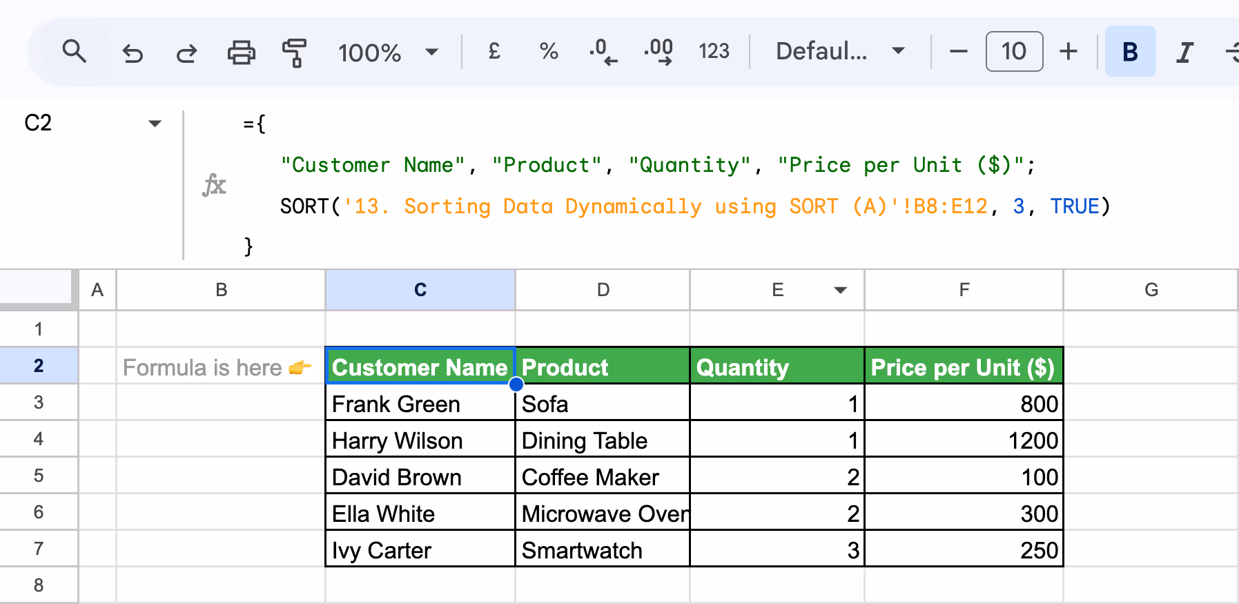
Sheet 1: Automatically Sorting Data using SORT (A)

In this sheet, we are sorting by price per unit in Descending Order.

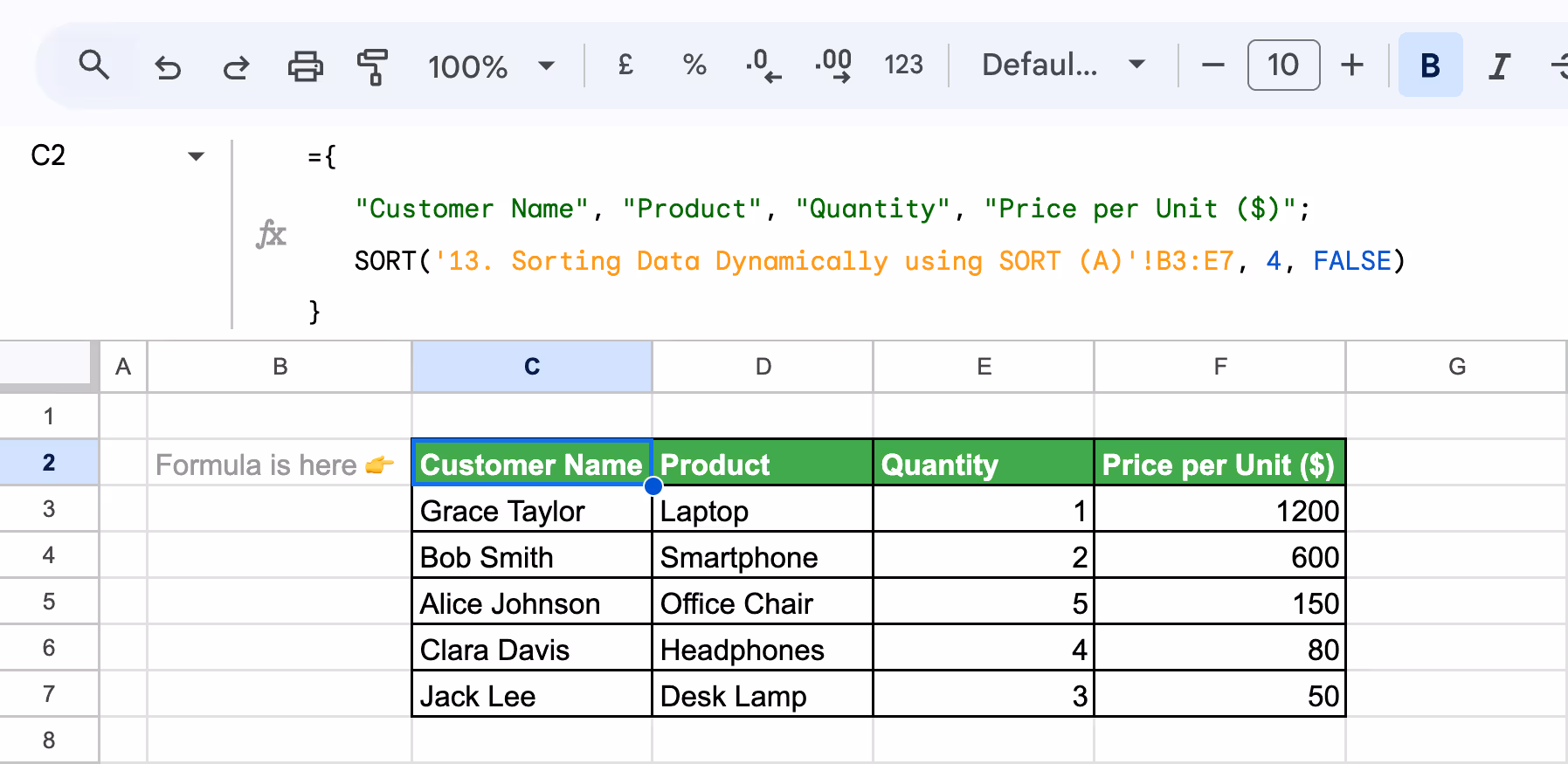
Use the following formula:

={
  "Customer Name", "Product", "Quantity", "Price per Unit ($)";
  SORT('Sorting Data Dynamically using SORT (A)'!B3:E7, 4, FALSE)
}

Here:

• "Customer Name", "Product", "Quantity", "Price per Unit ($)": Generates headers dynamically in the new sheet.
• SORT('Sorting Data Dynamically using SORT (A)'!B3:E7, 4, FALSE):
• B3:E7: Specifies the first chunk of the dataset 
• 4: Sorts by the Price per Unit ($) column (column index 4).
• FALSE: Sorts in descending order.

Sheet 2: Automatically Sorting Data using SORT (B)

In this new sheet, we are Sorting by Quantity in Ascending Order:

Enter the following formula:

={
  "Customer Name", "Product", "Quantity", "Price per Unit ($)";
  SORT('Sorting Data Dynamically using SORT (A)'!B8:E12, 3, TRUE)
}

Here:

• "Customer Name", "Product", "Quantity", "Price per Unit ($)": Generates headers dynamically in the new sheet.
• SORT('Sorting Data Dynamically using SORT (A)'!B8:E12, 3, TRUE):
• B8:E12: Specifies the second chunk of the dataset
• 3: Sorts by the Quantity column (column index 3).
• TRUE: Sorts in ascending order.

By using the SORT function, you can efficiently split and sort datasets into multiple sheets based on different criteria. 

Using the SORT Function to Reverse Rows

Reversing rows in Google Sheets can be achieved easily with the SORT function. If your dataset is unsorted, and you want to reverse its order without applying a specific sorting criterion, you can use this approach. 

Example: Reversing Rows in a Dataset

In this example, we’ll use the SORT function to reverse the rows in a dataset, starting with an unsorted dataset.

Use this formula:

={
  "Customer Name", "Product", "Quantity", "Price per Unit ($)";
  SORT(B3:E12, ROW(B3:E12), FALSE)
}

Here:

• "Customer Name", "Product", "Quantity", "Price per Unit ($)": Manually defined column headers for the output.
• SORT(B3:E12, ROW(B3:E12), FALSE):
• B3:E12: Range of the dataset.
• ROW(B3:E12): Provides row numbers as sorting criteria.
• FALSE: Sorts rows in descending order, reversing the dataset.

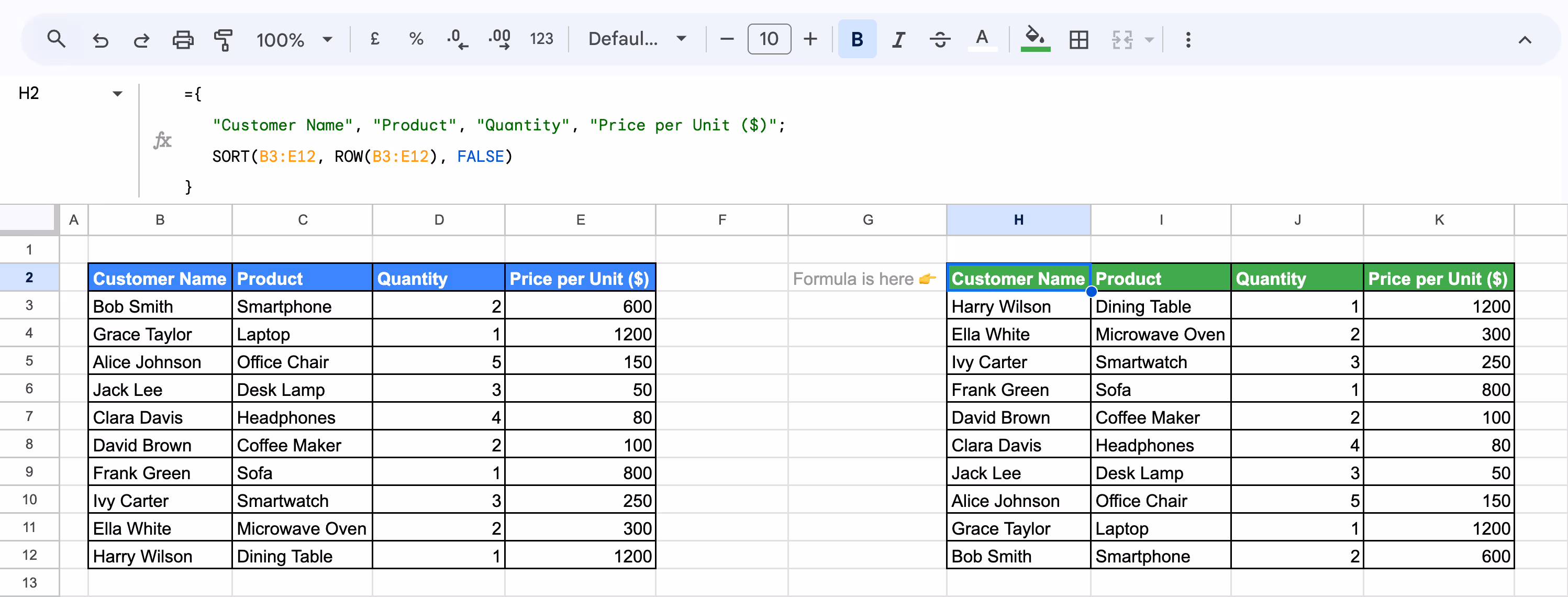
By using the SORT function with the ROW function, you can efficiently reverse the order of rows in your dataset, without applying any specific sorting logic.

Reversing Data with the INDEX and ROWS Functions

The INDEX and ROWS functions provide an alternative way to reverse rows in Google Sheets. This method dynamically retrieves rows in reverse order without relying on the SORT function

Example:

In this example, we’ll use these functions to reverse a dataset row by row.

Use this formula below:

=INDEX($B$3:$E$12, ROWS(B3:$E$12))

Here:

• =INDEX($B$3:$E$12, ROWS(B3:$E$12))$B$3:$E$12: The data range you want to reverse.
• ROWS(B3:$E$12): Calculates the number of rows in the range, starting from the last row and decreasing row-by-row as the formula is dragged down.

The combination of INDEX and ROWS offers a straightforward way to reverse rows manually, row-by-row.

Troubleshooting Challenges while Sorting Data in Google Sheets

Sorting data in Google Sheets isn't always seamless, as issues like inconsistent data types, blank cells, or improperly sorted headers can arise. Addressing these challenges ensures accurate organization and prevents errors in your analysis.

Sorting Not Working Due to Inconsistent Data Types

⚠️ Error: Sorting isn’t working due to inconsistent data types. Columns containing a mix of numbers and text-like numbers (e.g., "123" and "456 units") prevent Google Sheets from sorting correctly because it cannot interpret the values uniformly.

✅ Solution: Fix this issue by using the VALUE function to convert text-like numbers into numeric values. Wrap it with IFERROR to handle potential errors during conversion. 

Use this formula:

=IFERROR(VALUE(A2))

This ensures consistent data types, allowing seamless sorting in Google Sheets.

Fixing Blank Cells Sorted to the Top or Bottom

⚠️ Error: Blank cells are sorted to the top or bottom because Google Sheets treats them as having a value of 0 by default. This can disrupt the desired order of your dataset during sorting.

✅ Solution: To fix this, click on Data > Sort Sheet by and uncheck the option for "Treat empty cells as 0" in the sorting dialog. This ensures that blank cells are excluded from the sorting logic, maintaining a cleaner dataset.

Case-Sensitive Sorting Issues

⚠️ Error: Sorting is case-sensitive in Google Sheets, meaning text values like "apples" and "Apples" are treated differently during sorting. This can lead to incorrect or unexpected order in your dataset.

✅ Solution: To resolve this, use the LOWER function to standardize all text values to lowercase before sorting. Apply this formula in a helper column:

=LOWER(A2)

Once standardized, sort the dataset based on the new column for consistent, case-insensitive sorting.

Date Sorting Issues in Google Sheets

⚠️ Error: Sorting by date isn’t working because the date values are inconsistently formatted or not recognized as valid dates in Google Sheets. This prevents proper chronological sorting.

✅ Solution: Standardize date formatting by highlighting the column and selecting Format > Number > Date. If your dates are generated using a formula, wrap them in the DATEVALUE function to convert them into a recognized date data type. This ensures accurate sorting based on chronological order.

Not Checking for Headers When Sorting

⚠️ Error: Not checking for headers when sorting causes headers to be treated as regular data. This results in your column labels being misplaced within the dataset during sorting.

✅ Solution: Before sorting, select Data > Sort range > Advanced range sorting options and check the box for "Data has header row." This excludes the headers from the sorting process, keeping your dataset organized and easy to read.

Overlapping Filters Causing Confusion

⚠️ Error: Overlapping filters cause confusion in Google Sheets, as multiple filters applied to intersecting ranges can lead to unexpected behavior and incorrect sorting or filtering results.

✅ Solution: Ensure your filter ranges are distinct and do not overlap. Clear any existing filters by selecting Data > Remove filter before applying a new one. This avoids conflicts and ensures accurate filtering and sorting within the intended range.

Best Practices for Sorting Data in Google Sheets

Sorting data effectively in Google Sheets requires careful preparation to avoid errors and maintain data integrity. Following best practices ensures your datasets are well-organized, easy to navigate, and ready for analysis.

Keep Your Headers Consistent for Easy Sorting

Consistent headers make sorting and filtering effortless. Use clear, descriptive titles for each column, ensuring no duplicates or vague labels. Proper headers help Google Sheets identify the structure of your data, preventing errors and simplifying the process of organizing and analyzing your dataset effectively.

Use Conditional Formatting for Visual Cues

Conditional formatting highlights important data points automatically, providing instant visual cues for trends, outliers, or specific conditions. Apply rules to color-code rows or cells based on values, such as top-performing products or overdue tasks. This simplifies sorting and helps identify key insights at a glance.

Freeze Rows and Columns for Better Navigation

Freezing rows and columns ensures headers and critical data stay visible as you scroll through large datasets. To freeze, go to View > Freeze and select the rows or columns you want. This improves navigation and makes sorting or filtering large sheets more efficient and user-friendly.

Save Filter Views for Quick Access

Filter views let you save customized sorting or filtering preferences without altering the primary dataset. To create one, go to Data > Filter views > Create new filter view. These saved views make switching between different filtered results easy for quick data analysis.

Use Named Ranges for Durable Data References

Named ranges simplify working with formulas and improve data organization. Assign names to critical ranges via Data > Named ranges. Instead of cell references, use meaningful names in formulas, ensuring clarity and reducing errors when sorting or analyzing datasets. Named ranges also stay intact when data is updated.

Advanced Google Sheets Formulas for Precise Data Analysis

Efficient data analysis in Google Sheets requires leveraging advanced formulas tailored to tackle specific tasks. 

These powerful functions streamline your workflow and enable you to easily extract meaningful insights from complex datasets.

• IMPORTRANGE: Imports a range of cells from another Google Sheets file to combine data seamlessly.
• MATCH: Finds the position of a specific value within a defined range.
• MAX, MIN, MEDIAN: Calculates the highest, lowest, and median values in your dataset for comparative analysis.
• TIME: Converts hour, minute, and second values into a valid time format for scheduling or tracking purposes.
• REGEX: Validates, extracts, or replaces patterns in text using regular expressions, enabling efficient text manipulation and cleanup in datasets.
• ROUND: Rounds numbers to the desired decimal precision for accurate reporting.
• LEN: Counts the number of characters in a cell, including spaces, for precise data evaluation.

Visualize Your Data with OWOX: Reports, Charts & Pivots Extension

Transforming raw data into actionable insights is easier with the OWOX Reports extension for Google Sheets. This powerful tool enables you to create visually appealing reports and charts directly from your data, helping you identify trends, track performance, and make data-driven decisions. With its user-friendly interface, it’s perfect for analysts, marketers, and small business owners looking to simplify their workflows.

In addition to its intuitive design, OWOX offers advanced pivot table functionality, allowing you to organize and summarize data effortlessly. You can filter, sort, and analyze key metrics in seconds, saving time and reducing errors. Whether you're preparing a presentation or tracking KPIs, OWOX ensures your data is not only organized but also ready to impress stakeholders.