
Understanding the PERCENTRANK Function in Google Sheets: Rank Data by Percentile
Learn how to effectively apply the PERCENTRANK function in Google Sheets with practical examples, insights on .INC vs .EXC differences, and more.

Working with data can sometimes feel overwhelming, but the right tools make it much easier. Google Sheets provides powerful functions like PERCENTRANK that help you analyze and interpret data with precision. This function allows you to rank values by their relative percentile, offering deeper insights into your dataset.
Whether you're comparing performance, identifying trends, or segmenting data, PERCENTRANK turns raw numbers into actionable information.
In this article, we’ll show you how to use the PERCENTRANK function for accurate analysis, complete with real-world examples and best practices. Let’s explore how you can harness this function to make smarter, data-driven decisions in Google Sheets!
The Purpose of the PERCENTRANK Function in Google Sheets
The PERCENTRANK function in Google Sheets is designed to help you understand the relative standing of a value within a dataset. It calculates the percentile rank of a specific value, returning a number between 0 and 1 to indicate its position compared to other values.
This function is especially useful for performance tracking, comparing individual results within a group, or analyzing data distribution. For example, in student test scores, PERCENTRANK can show where a particular score falls compared to the rest.
By identifying these relative positions, you can easily detect patterns, identify outliers, and make informed decisions based on data rankings, ensuring more accurate and meaningful analysis.
Understanding the PERCENTRANK Function: Syntax and Examples
The PERCENTRANK function in Google Sheets helps determine the relative position of a value within a dataset as a percentile. This is useful for comparing data points and understanding how a value ranks among others. With simple syntax, the function provides quick insights into data distribution, making it easier to analyze performance or trends.
PERCENTRANK
The PERCENTRANK formula in Google Sheets calculates the percentage rank of a specified value within a dataset. It shows the percentage of values in the range that are less than or equal to the given value, making it useful for determining a value's relative position in statistical analysis.
Syntax of PERCENTRANK
The syntax of the PERCENTRANK function in Google Sheets is:
=PERCENTRANK(data, value, [significant_digits])
Let’s break down what these parameters represent:
- data: The range or array containing the dataset to analyze.
- value: The value for which you want to determine the percentage rank.
- significant_digits: (Optional) Specifies the number of significant digits to use in the result, defaulting to 3 if not provided.
Each of these parameters helps determine the relative rank of a value within the dataset.
Example of PERCENTRANK
Using the same monthly sales data, let's calculate the percentile rank for a sales figure, such as $42,500, to assess its relative position within the dataset.
Formula explanation:
=PERCENTRANK(C3:C12, 42500)
- C3:C12 Refers to the range containing sales data for all products.
- 42500: Represents the sales figure for which you want to calculate.
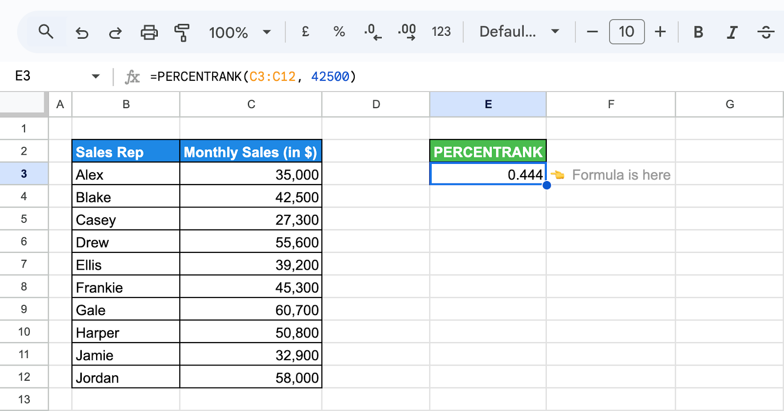
In cell E3, the formula will return 0.444, meaning it ranks in the 44.4th percentile within this dataset percentile. This value shows that 44.4% of the sales figures are less than or equal to $42,500, giving your business insight into where this sales figure stands relative to others in the dataset.
PERCENTRANK.INC
In Google Sheets, PERCENTRANK and PERCENTRANK.INC functions the same way, calculating the percentage rank of a value within a dataset. PERCENTRANK remains for backward compatibility, as older spreadsheet versions only had PERCENTRANK before the more specific. The variants – .INC and .EXC were introduced.
PERCENTRANK.EXC
PERCENTRANK.EXC in Google Sheets is a statistical function that calculates the percentile rank of a value within a dataset, excluding the boundary values. It determines the percentage of data points strictly less than the given value.
Unlike PERCENTRANK.INC, PERCENTRANK.EXC excludes the lowest and highest values, providing a more refined percentile rank by focusing on the data’s inner range.
Syntax of PERCENTRANK.EXC
The syntax of the PERCENTRANK.EXC function in Google Sheets is:
=PERCENTRANK.EXC(data, value, [significant_digits])
Let’s break down what these parameters represent:
- data: The range or array containing the dataset to analyze.
- value: The value for which you want to calculate the percentage rank.
- significant_digits: (Optional) The number of significant digits to include in the result, with 3 being the default if not specified.
These parameters help calculate the percentile rank while excluding boundary values from the dataset.
Example of PERCENTRANK.EXC
With the same monthly sales data, let's calculate the percentile rank for a specific figure, like the value in D3, to see how it compares to other sales figures in the dataset.
Formula explanation:
=PERCENTRANK.EXC(C3:C12, D3)
- C3: C12: Refers to the range containing sales data for all products.
- D3: Represents the specific sales value for which you want to calculate the percentile rank.
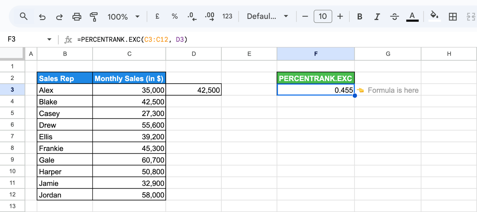
In cell F3, the formula will return the percentile rank of 0.455 relative to the sales data in C3, excluding boundary values. This result helps you assess how the sales figure in D3 compares to the rest of the dataset, providing a clearer picture of performance.
Practical Use Cases for PERCENTRANK Functions
PERCENTRANK functions are widely used for performance benchmarking, sales analysis, market research, academic assessments, and financial data interpretation. Here are some practical use cases of PERCENTRANK in Google Sheets.
Using PERCENTRANK.INC and PERCENTRANK.EXE with a Range of Cells
By using PERCENTRANK.INC and PERCENTRANK.EXC functions with a range of cells; you can easily calculate the percentile rank of any data point, allowing for more precise performance evaluations and comparisons.
Using PERCENTRANK.INC with a range of cells
Suppose you have monthly sales figures in column C; we will determine the percentile rank of a specific sales figure with PERCENTRANK.INC to understand its position within the dataset.
Formula explanation:
=PERCENTRANK.INC(C3:C12, 42500))
- C3:C12: Refers to the range of sales figures for all 10 sales representatives.
- 42500: Represents the sales figure for which you want to find the percentile rank.

In column E3, the formula will return 0.444, which is the percentile rank of a specific sales figure.
Using PERCENTRANK.EXC with a range of cells
Now again with the same list of monthly sales figures, this time you want to calculate the percentile rank of a specific sales figure using the exclusive version, PERCENTRANK.EXC.
Formula explanation:
=PERCENTRANK.EXC(C17:C26,42500)
- C16:C25: Refers to the range containing the sales data for all 10 sales representatives.
- 42500: The specific sales figure for which you want to calculate the percentile rank.

The formula returns 0.455 in column E16, which is the percentile rank of a specific sales figure.
Using PERCENTRANK.INC and PERCENTRANK.EXE with an Array
Using PERCENTRANK.INC and PERCENTRANK.EXE functions with an array of data allow you to quickly calculate the percentile rank of any specific value, making it easier to evaluate performance and make accurate comparisons.
Using PERCENTRANK.INC with an array
Let's say you have a small team of sales representatives whose monthly sales figures are {35,000; 42,500; 27,300; 55,600; 39,200; 45,300; 60,700; 50,800; 32,900; 58,000}. You want to find the percentile rank of a sales rep who achieved $55,600 to understand how their sales performance compares to others in the group.
Formula explanation:
=PERCENTRANK.INC(C3:C12, 55600)
- C3:C12: Refers to the range containing the performance scores for all employees.
- 55600: Represents the specific sales figure for which you want to calculate the percentile rank.
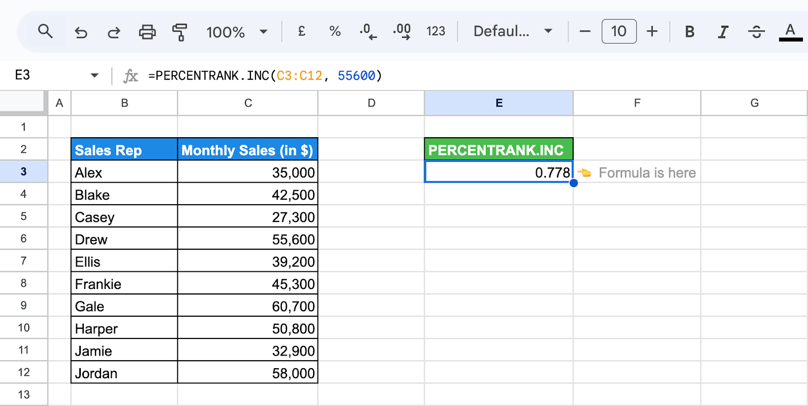
This means that $55,600 ranks at the 77.8th percentile within the dataset, indicating that 77.8% of the sales figures are less than or equal to $55,600.
Using PERCENTRANK.EXC with an array
With the same team’s monthly sales data, we will use PERCENTRANK.EXC to find the percentile rank of a rep with $55,600 in sales, highlighting how their performance compares within the group.
Formula explanation:
=PERCENTRANK.EXC(C15:C24, 55600)
- C15:C24: Refers to the range containing the performance scores for all employees.
- 55600: Represents the specific sales figure for which you want to calculate the percentile rank.

The formula will return 0.727, meaning that $55,600 ranks at the 72.7th percentile, excluding boundary values.
Finding Percentile Rank with Rounded Results Using PERCENTRANK.INC
Combining PERCENTRANK.INC with the ROUND function provides rounded percentile ranks, making the results more concise and easier to interpret for analysis or reporting. This method is useful when precise ranks are not needed.
Using the team’s monthly sales figures in Google Sheets, calculate the percentile rank of a specific rep’s sales, rounding the result to two decimal places for clarity in reporting.
Formula explanation:
=PERCENTRANK.INC(C3:C12, C4, 2)
- C3:C12: Refers to the range containing the sales figures.
- C4: Refers to the sales figure (8000) for which you want to find the percentile rank.
- 2: Rounds the result to two decimal places.

The percentile rank of 0.44 means that the sales figure in cell C4 is in the 44th percentile, indicating that 44% of the sales figures are less than or equal to this value.
Using PERCENTRANK for Comparative Data Analysis
PERCENTRANK aids in comparative data analysis by ranking values within a dataset. It allows businesses to easily compare performance and identify trends, which helps them make informed decisions and spot areas for improvement.
Using the dataset of monthly sales figures, let's calculate the percentile rank of a specific sales figure to understand how it compares to the rest.
Formula explanation:
=PERCENTRANK(C3:C12, 32900)
- C3:C12: Refers to the range containing the sales figures for all 10 sales reps.
- 32900: Refers to the specific sales figure (in this case, $32,900) whose percentile rank you want to calculate.

This formula will return a percentile rank of approximately 0.111, indicating that $32,900 ranks at the 11th percentile.
Resolving Common Issues with the PERCENTRANK Function in Google Sheets
When using the PERCENTRANK function in Google Sheets, common issues can arise, such as errors or unexpected results. These problems are often due to incorrect inputs or missing data. Reviewing your dataset and ensuring values are properly formatted can help resolve these issues and improve the accuracy of your analysis.
Invalid Range
⚠️ Error: The Invalid Range error in PERCENTRANK.EXC and PERCENTRANK.INC occurs when the dataset is empty, contains non-numeric values, or if the range reference is incorrect.
✅ Solution: Ensure the dataset includes valid numeric values and that the referenced range is correct. Check that the range is not empty, and remove any non-numeric entries. Double-check your formula to confirm the proper reference to the data range.
Inconsistent Data Types
⚠️ Error: The Inconsistent Data Types error in PERCENTRANK.EXC and PERCENTRANK.INC occurs when the dataset contains a mix of numeric and non-numeric values, preventing the function from calculating the percentile rank.
✅ Solution: Ensure the dataset contains only numeric values. Remove any text or non-numeric entries from the range. Verify your data for consistency to avoid errors before applying the formula.
Out-of-range Value
⚠️ Error: The Out-of-range Value error occurs in PERCENTRANK.INC and PERCENTRANK.EXC, when the value you're trying to rank is outside the range of the dataset, or the "k" value (percentile), is outside the valid range (less than 0 or greater than 1).
✅ Solution: Ensure your rank value is within the dataset's range. For percentile values, make sure the "k" argument is between 0 and 1. Double-check the dataset and the formula inputs for accuracy.
Omitting Value Parameter
⚠️ Error: The Omitting Value Parameter error in PERCENTRANK.INC occurs when a required parameter, such as the data range or percentile value, is missing. This prevents the function from calculating the percentile rank correctly.
✅ Solution: Ensure all necessary parameters are included in the formula. Double-check that the data range and percentile value are properly entered and that no arguments are left blank.
Best Practices for Effectively Using the PERCENTRANK Function in Google Sheets
To use the PERCENTRANK function effectively in Google Sheets, start with well-organized data and verify your inputs for accuracy. Ensure consistency in your dataset and check your results for reliability. Applying best practices helps improve your analysis and ensures more meaningful insights from your data.
Ensure Data Accuracy and Organization
Ensure data accuracy and organization when using the PERCENTRANK function in Google Sheets for reliable results. Remove non-numeric values, verify the completeness of your dataset, and ensure the range is correctly referenced. Consistent and clean data helps avoid errors and provides more accurate percentile rankings for better analysis.
Understand the Context of Your Data
Understanding the context of your data is essential when using the PERCENTRANK function in Google Sheets. Consider the data’s purpose, distribution, and scale to interpret percentile ranks accurately. Knowing how each value fits within the dataset helps you make more informed decisions and spot meaningful patterns or outliers.
Experiment with Different Data Ranges
Experimenting with different data ranges when using the PERCENTRANK function helps you gain deeper insights. Analyze specific subsets of your dataset to focus on particular periods, categories, or conditions. This approach allows you to identify trends, compare rankings, and make more targeted decisions based on refined data.
Use the Significance Parameter for Precise Results
Use the significance parameter in the PERCENTRANK function to achieve precise results. It determines the number of decimal places in the output, allowing for more accurate percentile rankings. Adjusting the significance level helps refine your analysis, especially when comparing closely ranked values within large datasets.
Verify Your Results with Cross-Checks
It's essential to verify your results using alternative methods or visual tools like charts and graphs. Cross-checking calculations ensures accuracy and reliability, helping you detect inconsistencies or errors early on and make more confident data-driven decisions.
Powerful Google Sheets Functions for Enhanced Data Analysis
Learn the full power of Google Sheets, with essential functions tailored for comprehensive data analysis. These advanced formulas simplify complex tasks, enabling you to handle large datasets, automate processes, and extract valuable insights effortlessly.
- SUM, SUMIF, and SUMIFS: Adds values from a range, with SUMIF and SUMIFS allowing conditional summing based on one or multiple criteria, simplifying targeted calculations.
- UNIQUE: Removes duplicates, providing a list of distinct values for cleaner analysis and identifying unique data points.
- PIVOT: Automatically summarizes data with pivot tables, helping you report, organize, and visualize trends effortlessly.
- IMPORTRANGE: Imports data from external Google Sheets, consolidating multiple sources into one, streamlining your data analysis.
- MATCH: Finds the position of a value within a range, useful for dynamic lookups when combined with other functions like INDEX.
- COUNTA: Counts non-empty cells in a range, giving a quick overview of your dataset’s size and density.
- MAX, MIN, MEDIAN: Returns the highest, lowest, and middle values in a dataset, providing insights into data distribution and central tendency.
- AVERAGE: Calculates the mean of a set of numbers, highlighting central trends and performance averages in your data.
Effortlessly Analyze Your Data with OWOX: Reports, Charts, and Pivot Tables
OWOX makes data analysis easy by transforming complex data into actionable insights. With advanced reports, charts, and pivot tables, it helps you visualize trends, identify patterns, and make smarter decisions. Managing large datasets becomes seamless, enabling you to find answers quickly.
Customizable reports and filters enable you to focus on the metrics that matter most to your business. The intuitive interface ensures efficient workflows, saving time and enhancing the accuracy of your data analysis.
Frequently asked questions


Finally, a tool that doesn't ask business users to learn a new dashboarding UI. Our marketing team already knows Sheets. OWOX just delivers the right data.
Joinable data marts concept was the thing that sold us. We can now use the semantic layer without building one.
Self-hosted the OSS version on Digital Ocean. Zero vendor lock-in. Contributed a Shopify connector back in week two.