
Mastering the RANK Function in Google Sheets: Rank Values Like a Pro
Learn how to effectively apply the RANK function in Google Sheets with practical examples, different ranking methods, and more tips for accurate data analysis.

Effectively analyzing your data can feel overwhelming, but the right tools make it much easier. Google Sheets provides powerful functions like RANK, allowing you to compare values, track performance, and organize data efficiently.
Whether you're ranking sales figures, exam scores, or performance metrics, the RANK function helps transform raw numbers into meaningful insights.
In this article, we'll walk you through using the RANK function in Google Sheets, covering its syntax, handling ties, and applying best practices. You'll also learn real-world use cases to enhance your data analysis. Let’s dive in and explore how mastering the RANK function can help you make smarter, data-driven decisions!
The Purpose of the RANK Function in Google Sheets
The RANK function in Google Sheets is a powerful tool for determining the relative position of a value within a dataset. It helps compare numbers by assigning a rank, making it useful for identifying top or bottom performers, such as the highest sales figures or the lowest exam scores.
This function is particularly valuable for performance tracking, competition rankings, or financial analysis. Additionally, it allows you to rank values based on specific criteria and identify ties or duplicate values, which can be highlighted for further review.
Whether analyzing business performance, academic results, or any other numerical dataset, the RANK function provides a straightforward way to sort and prioritize data, making it an essential tool for effective decision-making and trend analysis.
Understanding the RANK Function: Syntax and Examples
The RANK function in Google Sheets helps determine the position of a value within a dataset. It is useful for comparing numbers, identifying patterns, and organizing data in a meaningful way. By ranking values, you can easily analyze performance, spot trends, and make informed decisions based on your data.
RANK
The RANK function in Google Sheets determines the rank of a specific value within a given dataset, with 1 being the highest. It’s useful for identifying top or bottom performers in large datasets. When ties occur, the function assigns the same rank to equal values, with subsequent ranks adjusted accordingly.
Syntax of RANK
The syntax of the RANK function in Google Sheets is:
=RANK(value, data, [is_ascending])
Let’s break down what these parameters represent:
- value: The value whose rank you want to determine.
- data: The range or array containing the dataset to compare the value against.
- is_ascending: (Optional) Specifies whether to rank in ascending (1) or descending (0) order. The default is descending (0), where 1 represents the highest rank.
This function allows you to rank values based on their position in the dataset.
Example of RANK
Let’s say you’re ranking sales reps by their performance, from highest to lowest, to see who leads in monthly sales.
Formula Explanation:
To rank the reps based on their sales figures, you can use the following formula
=RANK(C3, C$3:C$12, 0)
- C3: Refers to the cell containing the sales figure.
- C$3:$12: Refers to the range containing sales figures for all 10 Sales Reps.
- 0: Specifies that the ranking is in descending order (higher sales ranked first).
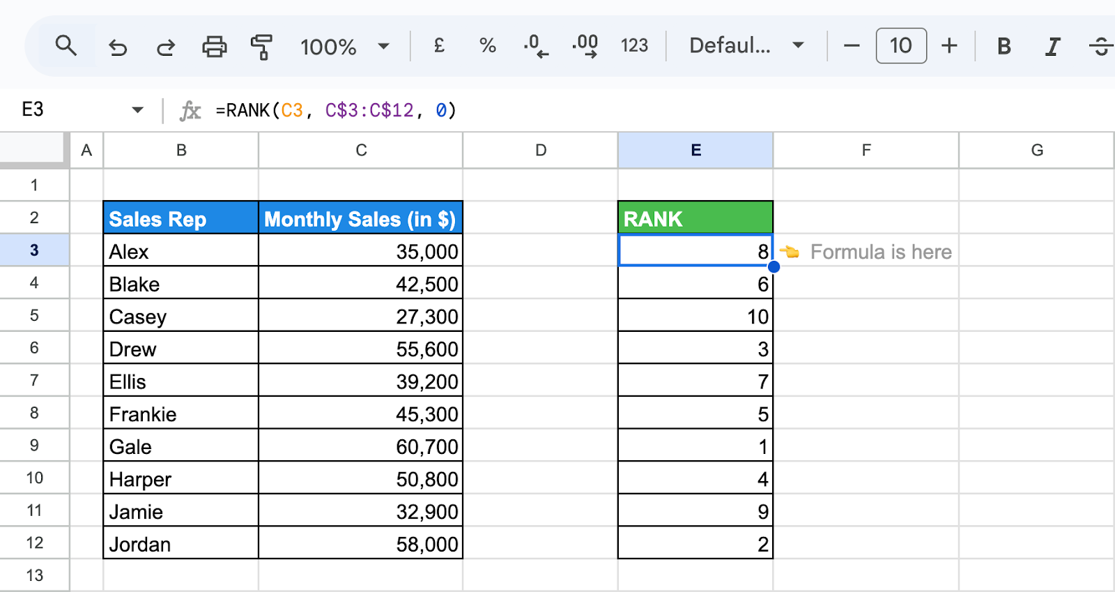
This formula will rank products in Column E based on their sales in descending order, with higher sales receiving a higher rank.
RANK.EQ
In Google Sheets, RANK.EQ is the modern replacement for the original RANK function. Both functions behave identically: they assign the same rank to equal values and skip the next rank positions when ties occur. The key difference is naming, not functionality.
Google introduced RANK.EQ to make ranking behavior more explicit and consistent with other ranking functions, such as RANK.AVG. While RANK is still supported for backward compatibility, it’s recommended to use RANK.EQ in new formulas. For this reason, all upcoming examples in this article will use RANK.EQ instead of RANK.
RANK.AVG
RANK.AVG is a function in Google Sheets that calculates the rank of a specified value in a dataset, averaging the ranks for tied values. This means when two or more values are equal, they receive the average rank instead of identical ranks.
Syntax of RANK.AVG
The syntax of the RANK.AVG function in Google Sheets is:
=RANK.AVG(value, data, [is_ascending])
Let’s break down what these parameters represent:
- value: The value whose rank you want to determine.
- data: The range or array containing the dataset to compare the value against.
- is_ascending: (Optional) Specifies whether to rank in ascending (1) or descending (0) order. The default is descending (0), where 1 represents the highest rank.
This function returns the average rank for tied values, providing a more balanced ranking system.
Example of RANK.AVG
Suppose now you’re ranking sales reps by performance and want to assign an average rank for any ties, ensuring a fair comparison among similarly performing reps.
Formula Explanation:
To rank the reps based on their sales figures, you can use the following formula:
=RANK.AVG(C3, C$3:C$12, 0)
- C3: Refers to the cell containing the sales figure.
- C$3:$12: Refers to the range containing sales figures for all 10 reps.
- 0: Specifies that the ranking is in descending order (higher sales ranked first).
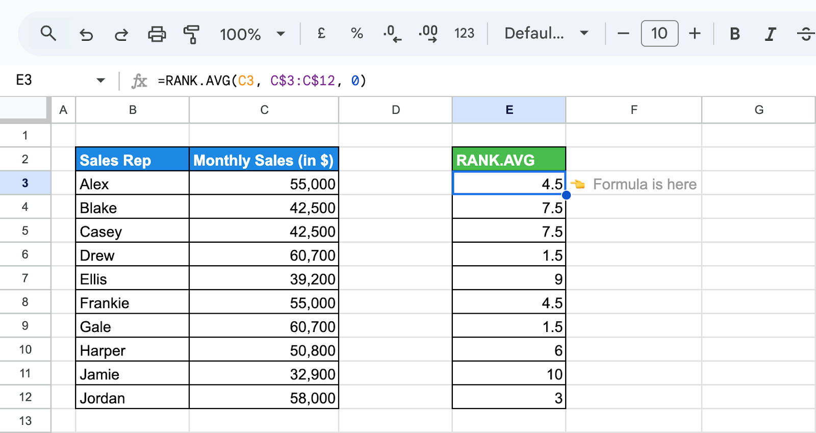
This formula will rank the reps in E based on their sales, assigning an average rank if any ties exist. This way, tied reps will receive an average of their ranks, providing a fair ranking system.
.png
)
Hands-On Examples of Using the RANK Function in Google Sheets
Whether you want to see who scored highest or lowest in a competition or just need to organize your data, the RANK function in Google Sheets can help by ranking values in ascending or descending order. Let's look at some real-world examples.
Ranking in Descending Order Using RANK.EQ Function
The RANK.EQ function in Google Sheets is a quick way to rank numbers in a list. If you want to rank values in descending order, setting the order to 0 ensures the largest number gets the top rank. This is handy when you need to sort sales figures or test scores, where higher values mean better performance. It’s an easy tool to organize your data and see who comes out on top.
Example of RANK.EQ
Using the same sales figures for your top reps, let's apply RANK.EQ to list each rep’s performance in descending order, identifying the highest performers.
Formula Explanation:
=RANK.EQ(C3, C3:C12, 0)
- C3:C12: represents all sales figures.
- 0: Represents the dataset to be arranged in Descending Order
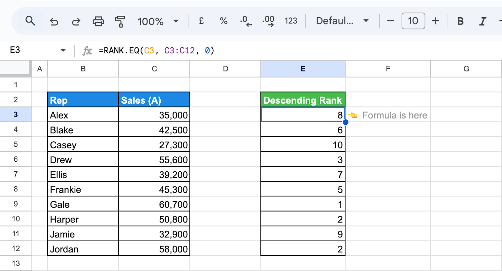
The 0 ranks them in descending order. In this case, Gale ranks 1st, giving you quick insight into sales performance.
Ranking with Ties Using the RANK.EQ and RANK.AVG Functions
When ranking data in Google Sheets, ties can occur when multiple values share the same rank. The RANK.EQ and RANK.AVG functions handle these ties differently. RANK.EQ assigns the same rank to tied values, while RANK.AVG gives them an average rank for fairness.
Example for RANK.EQ
Using the monthly sales data, now let's apply RANK.EQ to rank sales reps, assigning the same rank to those with identical sales figures.
Formula Explanation:
=RANK.EQ(C3, C$3:C$12)
- C3: Refers to the sales amount for Rep A.
- C$3:C$12: Refers to the range containing sales amounts for all reps.
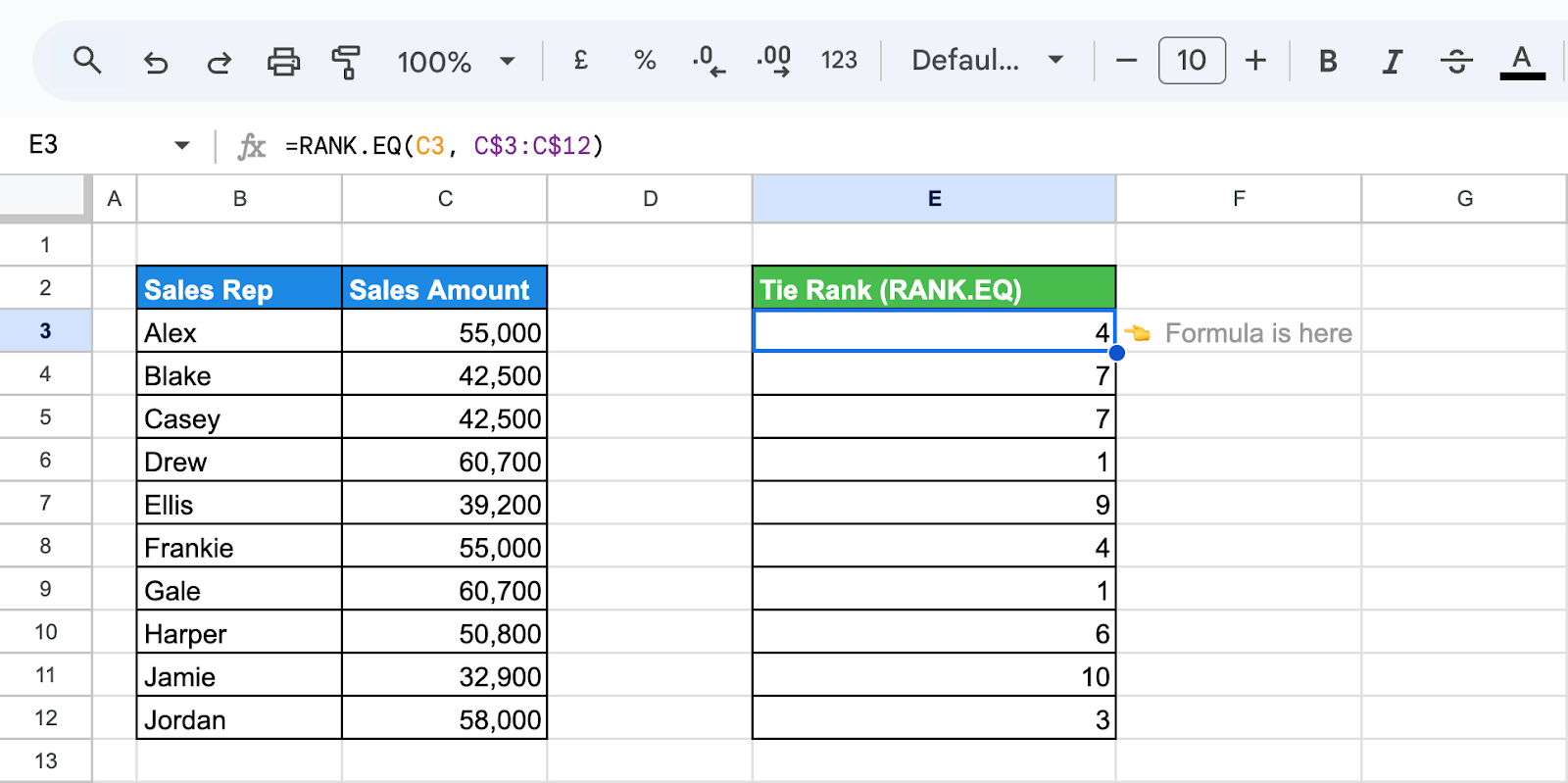
Both Drew and Gale have the same sales amount of $60,700, so RANK.EQ assigns both of them a rank of 1. The next highest sales amount will be ranked 3, skipping rank 2. This method ensures that ties are properly accounted for in ranking.
Example for RANK.AVG
Using the same monthly sales data, apply RANK.AVG to rank your team, ensuring that identical sales figures are assigned an average rank for balanced comparison.
Formula Explanation:
=RANK.AVG(C16, C$16:C$25)
- C16: Refers to the sales amount for Rep A.
- C$16:C$25: Refers to the range containing sales amounts for all sales reps.
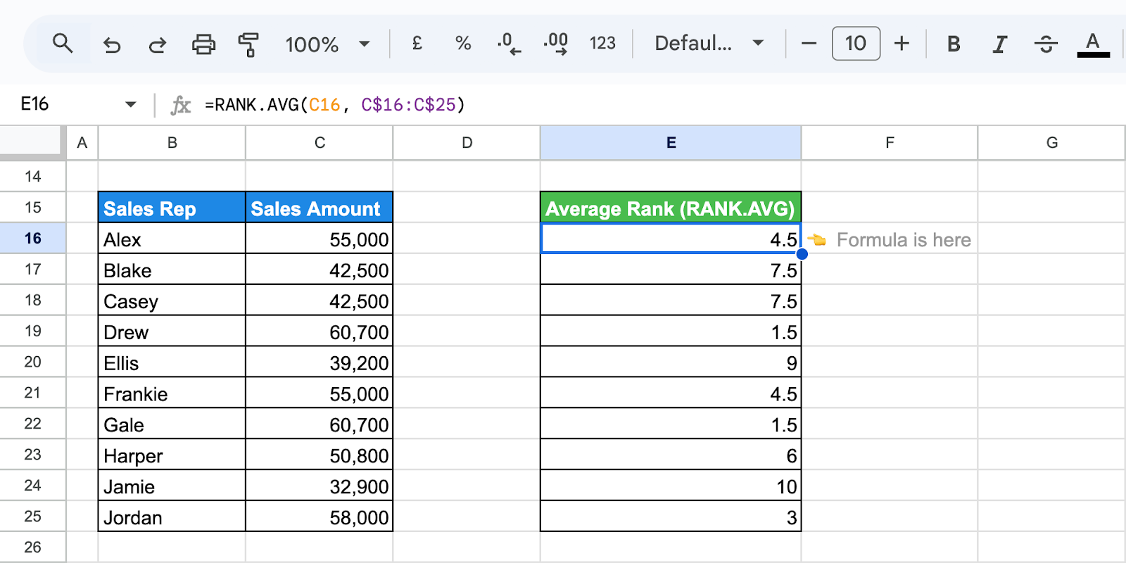
Since both Drew and Gale have the same sales figure of $60,700, RANK.AVG will assign both an average rank of 1.5. The next highest sales figure, $58000, will be ranked 3, maintaining fairness in ranking tied values.
Combining the RANK Function with Other Functions in Google Sheets
Combining the RANK function with other functions in Google Sheets enhances data analysis and organization. Using it with IF helps apply conditions, while COUNTIFS allows ranking within specific groups. Pairing it with AVERAGE or MAX can provide additional insights, making it easier to analyze trends, compare values, and draw meaningful conclusions from your data
Using ARRAYFORMULA with RANK.EQ and RANK.AVG Functions
In Google Sheets, ARRAYFORMULA allows you to apply a function over a range of values. When combined with RANK.EQ and RANK.AVG, you can rank data automatically across multiple cells without applying the formula one by one.
Example of ARRAYFORMULA with RANK.EQ
Suppose you want to rank each sales rep based on their monthly sales performance. Using ARRAYFORMULA with RANK.EQ allows you to rank all sales figures in one go.
Formula Explanation:
=ARRAYFORMULA(RANK.EQ(C3:C12, C3:C12, 0))
- ARRAYFORMULA: Applies the ranking function across the entire range at once.
- RANK.EQ(C3, C3, 0): Ranks each sales rep’s monthly sales figure in descending order, with the highest sales getting rank 1.
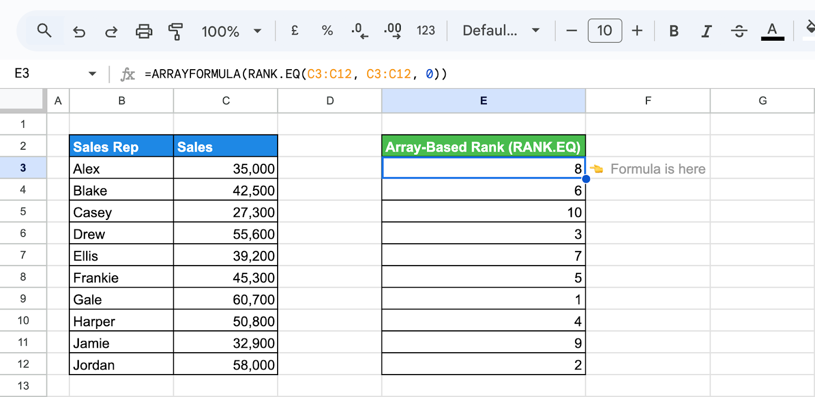
This formula will return the rank of each employee's sales without the need to apply the function manually row by row.
Example of ARRAYFORMULA with RANK.AVG
Now, let’s say you want to rank your sales reps, but account for any ties by using RANK.AVG, which assigns an average rank to tied values.
Formula Explanation:
=ARRAYFORMULA(RANK.AVG(C3:C12, C3:C12, 0))
- ARRAYFORMULA: Applies the formula across all rows in the range.
- RANK.AVG(C3, C3, 0): Ranks each sales rep’s monthly sales figure in in descending order, assigning average ranks to tied values.
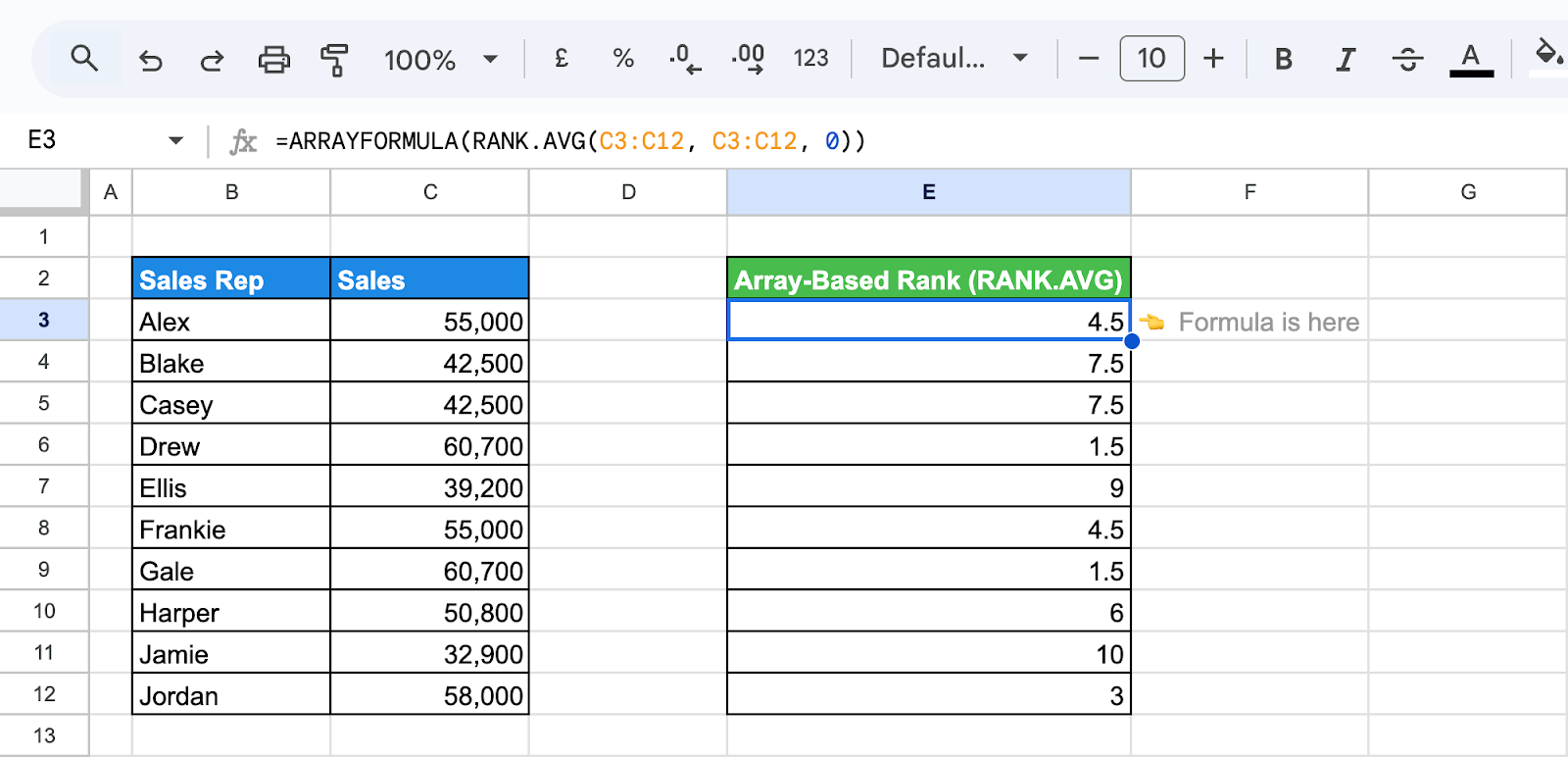
Like, for example, Drew and Gale both have sales of $60,700 and receive an average rank of 1.5. Alex and Frankie both have sales of $55,000 and receive an average rank of 4.5. Blake and Casey both have sales of $42,500 and receive an average rank of 8.5.
💡Now that you’ve explored using ARRAYFORMULA with RANK.EQ and RANK.AVG is for efficient data ranking, so why stop there? Discover even more ways to streamline your processes with ARRAYFORMULA in Google Sheets in our in-depth guide.
Resolving Common Issues with the RANK Function in Google Sheets
When using the RANK function in Google Sheets, you may encounter issues such as incorrect rankings, unexpected ties, or missing values. These problems often arise from data formatting errors or incorrect range selection. Ensuring clean, consistent data and verifying inputs can help improve accuracy and make rankings more reliable for analysis.
#VALUE!
⚠️ Error: The #VALUE! error in RANK.EQ and RANK.AVG occurs when the function is provided with non-numeric values or incorrect arguments. This prevents the function from ranking the data properly.
✅ Solution: Ensure that the dataset and the value being ranked contain only numeric values. Check that the rank parameters are correctly defined and that there are no text entries or empty cells in the range. If needed, convert non-numeric data or remove invalid entries to prevent errors.
#N/A Error
⚠️ Error: The #N/A error in RANK.EQ and RANK.AVG occurs when the dataset is empty, contains non-numeric values, or when the value being ranked is not found in the dataset.
✅ Solution: Ensure the dataset contains only numeric values and is not empty. Double-check that the value you’re trying to rank exists within the data range. If the dataset includes text or blank cells, clean the data by removing or correcting invalid entries.
Best Practices for Effectively Using the RANK Function in Google Sheets
To use the RANK function effectively in Google Sheets, ensure your data is well-organized and contains only numeric values. Verify that your range is correctly referenced, and consider handling ties appropriately. Combining RANK with other functions can enhance analysis, while cross-checking results helps ensure accuracy and meaningful insights.
Ensure Data Accuracy and Organization
Ensure data accuracy and organization when using the RANK function in Google Sheets for reliable results. Make sure your dataset contains only numeric values, remove any blank or non-numeric entries, and verify that the data range is correctly referenced. Well-structured data improves ranking accuracy and helps generate meaningful insights for better analysis.
Understand the Context of Your Data
Understanding the context of your data is crucial when using the RANK function in Google Sheets. Consider the dataset’s distribution, the presence of duplicate values, and whether you need ascending or descending rankings. Interpreting results within the right context helps ensure meaningful analysis and more accurate comparisons for decision-making.
Combine with Other Functions for Deeper Insights
Combining the RANK function with other functions in Google Sheets enhances data analysis and provides deeper insights. Use IF to apply ranking conditions, COUNTIFS to rank within specific groups, or AVERAGE to analyze ranked data trends. Integrating these functions helps refine rankings, identify patterns, and improve decision-making based on data comparisons.
Handle Ties and Special Cases Effectively
Handling ties and special cases effectively is essential when using the RANK function in Google Sheets. Use RANK.AVG to assign average ranks for duplicate values, or COUNTIF to adjust rankings dynamically. Consider sorting data appropriately and applying conditional formatting to highlight tied values for better analysis and decision-making.
Use Conditional Formatting for Better Visualization
Using conditional formatting with the RANK function in Google Sheets enhances data visualization by making rankings easier to interpret. Apply color scales to highlight top and bottom values, or use custom rules to emphasize specific ranks. This approach helps quickly identify trends, outliers, and key performance indicators within your dataset.
Experiment with Different Data Ranges
Experimenting with different data ranges when using the RANK function in Google Sheets can provide valuable insights. Analyze specific subsets of data, such as ranking within departments, time periods, or performance categories. This approach helps refine comparisons, highlight trends, and improve decision-making by focusing on relevant data within your dataset.
Verify Your Results with Cross-Checks
Validating your results with alternative methods or visual tools like charts and graphs is essential. Cross-checking calculations enhances accuracy and reliability, helping you identify inconsistencies or errors early. This ensures your analysis is precise and supports well-informed decision-making based on reliable data.
Powerful Google Sheets Functions for Enhanced Data Analysis
Learn the full power of Google Sheets, with essential functions tailored for comprehensive data analysis. These advanced formulas simplify complex tasks, enabling you to handle large datasets, automate processes, and extract valuable insights effortlessly.
- SUM, SUMIF, and SUMIFS: Adds values from a range, with SUMIF and SUMIFS allowing conditional summing based on one or multiple criteria, simplifying targeted calculations.
- UNIQUE: Removes duplicates, providing a list of distinct values for cleaner analysis and identifying unique data points.
- PIVOT: Automatically summarizes data with pivot tables, helping you report, organize, and visualize trends effortlessly.
- IMPORTRANGE: Imports data from external Google Sheets, consolidating multiple sources into one, streamlining your data analysis.
- MATCH: Finds the position of a value within a range, useful for dynamic lookups when combined with other functions like INDEX.
- COUNTA: Counts non-empty cells in a range, giving a quick overview of your dataset’s size and density.
- MAX, MIN, MEDIAN: Returns the highest, lowest, and middle values in a dataset, providing insights into data distribution and central tendency.
- AVERAGE: Calculates the mean of a set of numbers, highlighting central trends and performance averages in your data.
Effortlessly Analyze Your Data with OWOX: Reports, Charts, and Pivot Tables
OWOX Reports streamlines data analysis by transforming complex data into actionable insights. With advanced reports, charts, and pivot tables, it helps you visualize trends, identify patterns, and make data-driven decisions. Managing large datasets becomes effortless, allowing you to access key insights quickly.
Customizable reports and filters enable you to focus on the most critical business metrics. The intuitive interface enhances efficiency, saving time while ensuring precise and accurate data analysis.
Frequently asked questions


Finally, a tool that doesn't ask business users to learn a new dashboarding UI. Our marketing team already knows Sheets. OWOX just delivers the right data.
Joinable data marts concept was the thing that sold us. We can now use the semantic layer without building one.
Self-hosted the OSS version on Digital Ocean. Zero vendor lock-in. Contributed a Shopify connector back in week two.