
Optimizing Your Data with TRIM, CLEAN, and T Functions in Google Sheets
Master TRIM, CLEAN, and T Functions in Google Sheets to clean data, eliminate special characters, and enhance readability.

Efficient data management often requires the refinement of text data to ensure accuracy and usability in Google Sheets. The TRIM, CLEAN, and T functions are indispensable tools for anyone looking to polish and prepare text-based data for analysis.
TRIM removes extra spaces from text, CLEAN eliminates non-printable characters, and the T function helps differentiate text from non-text in your cells.
This guide will explore how to utilize these functions to maintain clean, streamlined data that enhances the clarity and effectiveness of your spreadsheets.
Whether you’re dealing with imported data, preparing reports, or simply organizing your datasets, learn how these functions can optimize your Google Sheets experience, making your data cleaner and your workflows smoother.
Why Data Cleanup is Crucial for Google Sheets Users
Data cleansing is an essential task that enhances the accuracy, consistency, and integrity of your data. Without diligent cleansing, you risk generating misleading reports, encountering workflow delays, and perpetuating errors across your analyses, which can negatively impact your decision-making. Moreover, clean data not only streamlines your processes but also bolsters the dependability of your insights.
Functions such as TRIM, CLEAN, and T are invaluable for removing extraneous characters, normalizing formatting, and arranging text. These tools help ensure that your data is meticulously prepped for analysis or reporting. By leveraging these functions, you can handle your data more effectively and confidently, ensuring it is devoid of errors and ready for use.
Exploring the TRIM, CLEAN and T Functions (With Syntax and Examples)
Enhance your text management skills in Google Sheets with these crucial functions. TRIM helps delete surplus spaces, CLEAN eradicates non-printable characters, and T facilitates text filtering. In this section, we will delve into the syntax and practical examples of the TRIM, CLEAN, and T functions, empowering you to refine your data cleaning and formatting abilities.
TRIM Function
The TRIM function is particularly useful for cleaning up data imported from external sources or ensuring consistency in text entries.
Syntax of TRIM
=TRIM(text)
Let's break down the parameters:
- text: The text string from which you want to remove extra spaces.
The TRIM function is useful for cleaning text, ensuring consistent spacing in your dataset.
Example of TRIM
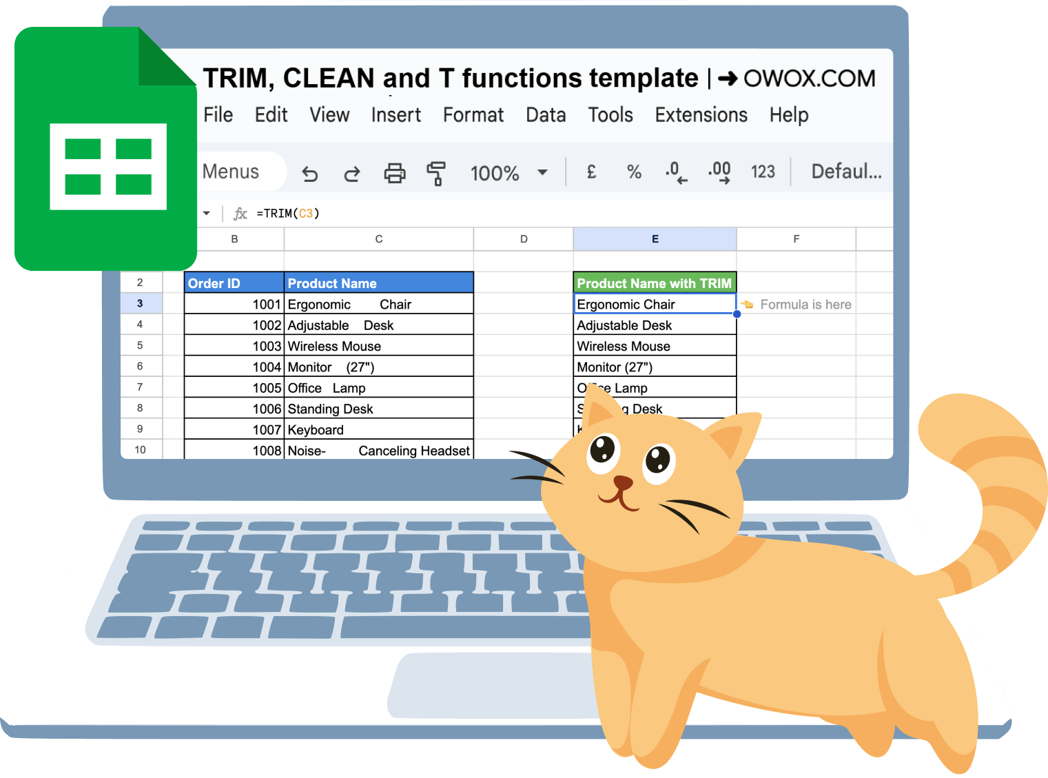
Let’s say you have Product Name details in column C with extra spaces, and you want to clean the text for consistency.
Syntax:
=TRIM(C3)

Here:
- C3: Refers to the cell containing the Product Name with extra spaces.
This formula removes unnecessary spaces from the text in column C and outputs the cleaned text in column E, ensuring only single spaces remain between words.
CLEAN Function
The CLEAN function in Google Sheets removes non-printable ASCII characters (codes 0 through 31) from text, ensuring data integrity. This is particularly useful when importing data from external sources containing hidden characters, which can disrupt analysis and reporting.
Syntax of CLEAN
CLEAN(text)
Let’s break down what these parameters represent:
- text: The text string you want to clean by removing non-printable characters.
The function is essential for ensuring your data is free of hidden or non-visible characters that may disrupt analysis or formatting.
Example of CLEAN
Let’s say you have Customer Feedback data in column C containing non-printable characters, and you want to clean the text for proper formatting.
Syntax:
=CLEAN(C3)
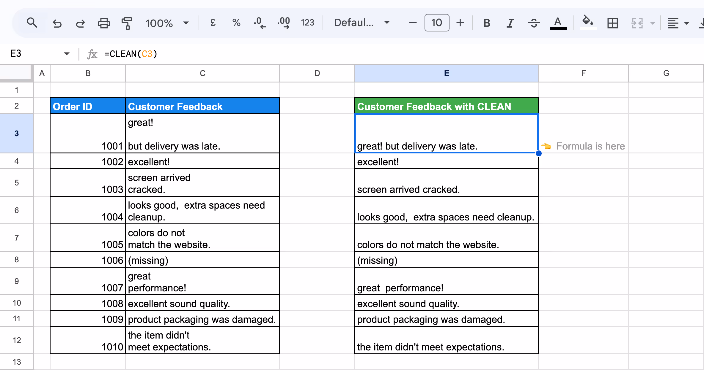
Here:
- C3: Refers to the cell containing the text with non-printable characters.
This formula removes all non-printable characters from the feedback in column C and outputs the cleaned text in column E, ensuring the feedback is ready for analysis or reporting.
T Function
The T function in Google Sheets evaluates whether a given value is text. If the value is text, it returns the text itself; otherwise, it returns an empty string. This function is handy for working with datasets containing mixed data types.
Syntax of T
T(value)
Let’s break down what this parameter represents:
- value: The value to check.
This function is useful for filtering text values from a dataset, ensuring only text is returned when working with mixed data types.
Example of T
Let’s say you have Customer Name data in column C, and you want to return the text values from it using the T function.
Syntax:
=T(C3)

Here:
- C3: Refers to the cell containing the Customer Name.
This formula checks the value in column C and returns the text if the cell contains text. If the cell contains anything else (e.g., a number or blank), it returns an empty string. The cleaned text appears in column E.
Simple Examples of Using TRIM, CLEAN and T Functions in Google Sheets
The functions TRIM, CLEAN, and T simplify data management in Google Sheets. Whether you're looking to eliminate unwanted spaces, clear non-printable characters, or filter cell content, these functions can streamline your tasks. In this section, we'll provide practical examples that show how each function operates and how it can enhance your spreadsheet workflows.
Using T Function for Handling Numbers and Booleans
The T function in Google Sheets filters out non-text values like numbers or booleans, returning an empty string.
Example:
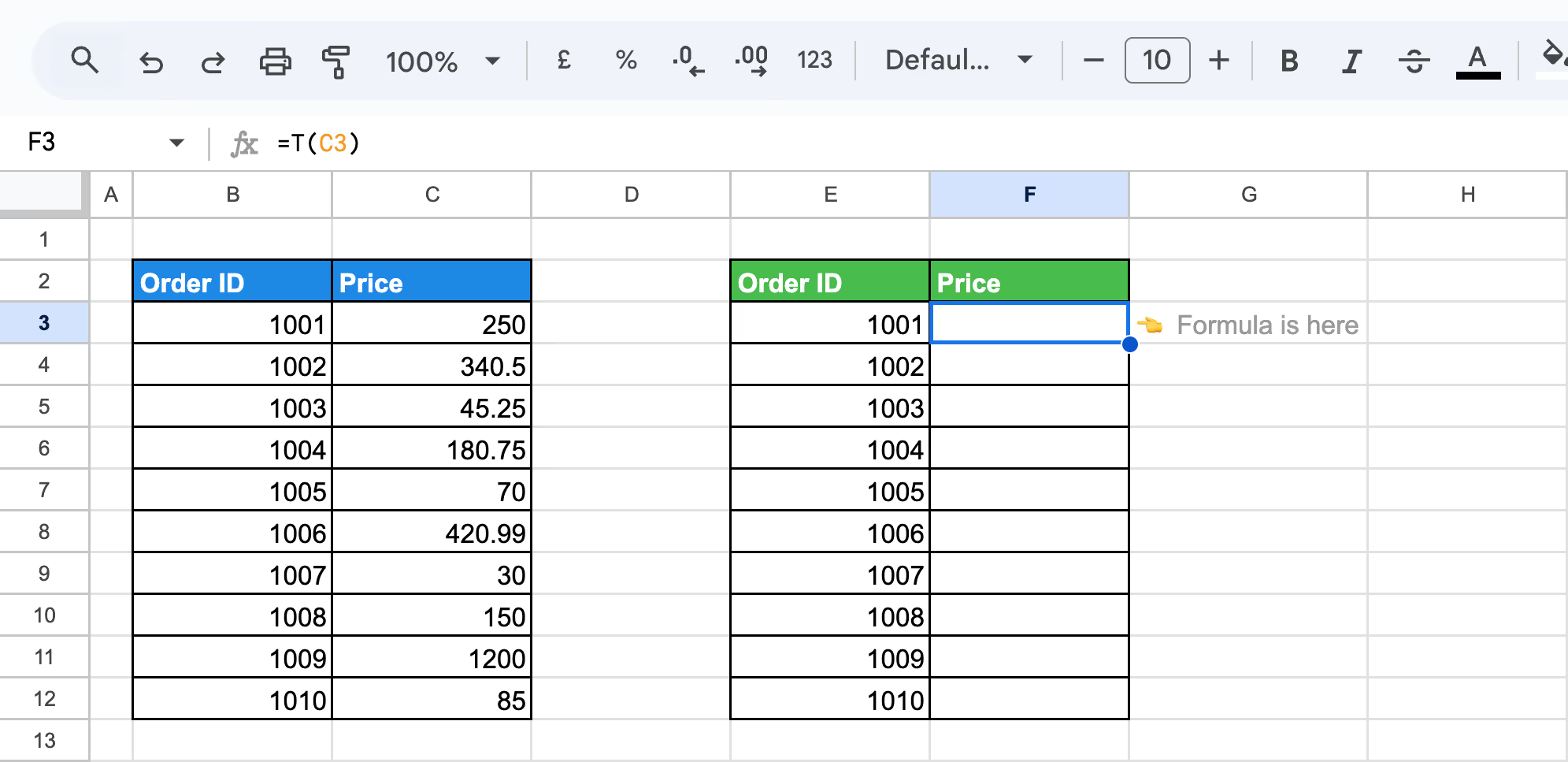
Let’s say you want to check if there is any non-text data in the Price column (C) and display results in column F for formatting purposes.
Use the following formula in a new cell:
=T(C3)
Here:
- C3: Refers to the cell containing the value to check.
This formula checks each value in column C. If the value is text, it is displayed in column F; otherwise, the cell remains blank. This simplifies data by removing unwanted numerical or boolean values.
Filtering Text Values Using the T Function
The T function in Google Sheets is particularly useful for preparing clean and readable lists for analysis. Let’s see how to use it for a mixed dataset.
Example:
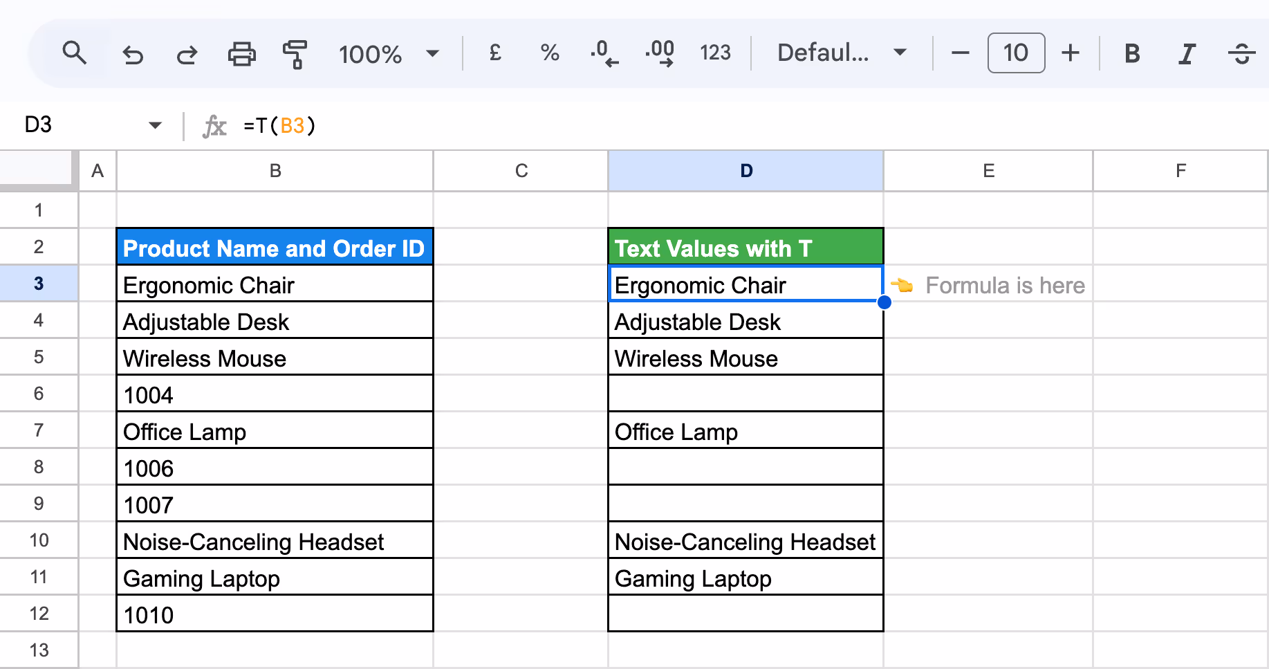
Let’s say you have a dataset in column B containing product names and order IDs in a haphazard manner, and you want to filter out the product names.
Use the following formula in a new cell:
=T(B3)
Here:
- B3: Refers to the cell containing the value to evaluate.
This formula checks each value in column B. Text values are displayed in column D, while non-text entries (like numbers) are left blank. This results in a clean list of product names for easy analysis.
Combining TRIM, CLEAN, and T Functions with Other Functions
Integrating the TRIM, CLEAN, and T functions with other Google Sheets functions can greatly improve your data cleaning and analysis efforts. This method facilitates more advanced operations, allowing you to streamline processes and maintain accurate, consistent datasets throughout your spreadsheets.
Combining ARRAYFORMULA with TRIM and CLEAN Functions
Combining ARRAYFORMULA with the TRIM and CLEAN functions in Google Sheets allows you to efficiently process and clean large datasets. The TRIM function removes extra spaces, while CLEAN eliminates non-printable characters.
Example of TRIM and ARRAYFORMULA:
Suppose you have a dataset where the Product Name column contains extra spaces between words. You can use the TRIM function in combination with ARRAYFORMULA to remove these extra spaces for the entire range.
Use this formula:
=ARRAYFORMULA(TRIM(C3:C12))

Here:
- TRIM(C3:C12): The TRIM function removes leading, trailing, and multiple spaces between words for each text value in the Product Name range.
- ARRAYFORMULA: The ARRAYFORMULA function allows the TRIM function to be applied to the entire range, automatically cleaning the text in all the cells in the range.
By using ARRAYFORMULA with TRIM, you can efficiently remove extra spaces from a range of cells, cleaning up your dataset for further analysis or presentation.
Example of CLEAN and ARRAYFORMULA:
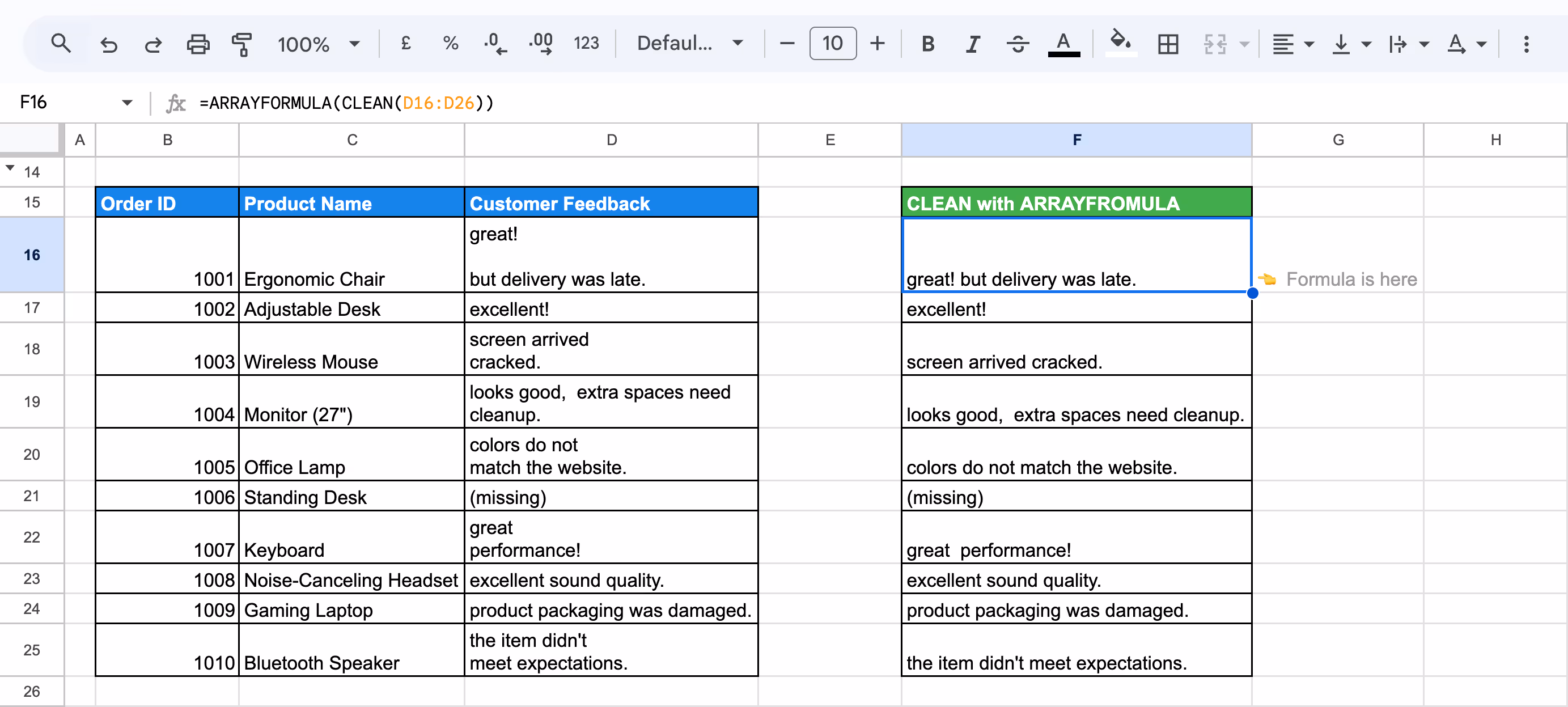
Suppose you have a dataset with Customer Feedback that contains unwanted line breaks, extra spaces, or non-printable characters. You can use the CLEAN function in combination with ARRAYFORMULA to remove these characters and clean the feedback text.
Use this formula:
=ARRAYFORMULA(CLEAN(D16:D26))
Here:
- CLEAN(D16:D26): The CLEAN function removes non-printable characters such as line breaks, tabs, and other invisible formatting characters from the Customer Feedback range.
- ARRAYFORMULA: The ARRAYFORMULA function allows the CLEAN function to be applied to the entire range, automatically cleaning the text in all cells from D16 to D26.
Using ARRAYFORMULA with the CLEAN function, you can easily remove line breaks from an entire range of feedback text, ensuring consistency and improving data quality.
Removing HTML Tags with CLEAN and REGEXREPLACE
The CLEAN function in Google Sheets helps remove unwanted characters, including non-printable ones often introduced by HTML tags. This ensures the data is clean and easy to read, especially when importing from external sources like websites. CLEAN simplifies data cleaning, leaving only plain, usable text for analysis or presentation.
Example:
Let’s say you have raw data in column C with HTML tags and unnecessary characters. You want to clean it for better readability and use it in column E.
Use the following formula in a new cell:
=CLEAN(REGEXREPLACE(C3, "<[^>]+>", ""))

Here:
- C3: Refers to the cell containing the raw data with HTML tags.
- REGEXREPLACE(C3, "<[^>]+>", ""): Strips out HTML tags using a regular expression.
- CLEAN: Removes any leftover non-printable characters.
This formula cleans up the raw data, leaving clear, usable text in column E, such as "$250.00 USD" or "Price: 85.00."
Eliminating Punctuation Using CLEAN and REGEXREPLACE
The CLEAN function in Google Sheets helps remove unwanted characters, including punctuation, ensuring the data is clean and easy to read. This simplifies data cleaning, leaving only plain, usable text for analysis or presentation.
Example:
Let’s say you have raw customer feedback in Column C with punctuation. You want to clean it for better readability and display the cleaned feedback in Column E.
Use the following formula in a new cell:
=CLEAN(REGEXREPLACE(C3, "[[:punct:]]", ""))

Here:
- C3: Refers to the cell containing the raw data with punctuation.
- REGEXREPLACE(C3, "[[:punct:]]", ""): Strips out punctuation using a regular expression.
- CLEAN: Removes any leftover non-printable characters.
This formula cleans up the raw data, leaving clear, usable text in Column E, such as "great performance" or "product packaging was damaged."
Combining ARRAYFORMULA, TRIM, and SPLIT for Cleaner Rows
ARRAYFORMULA, TRIM, and SPLIT in Google Sheets allow you to efficiently clean and separate data within a range. This approach is useful when removing extra spaces and splitting multiple values in a single cell into individual rows, ensuring cleaner and more organized data.
Example:
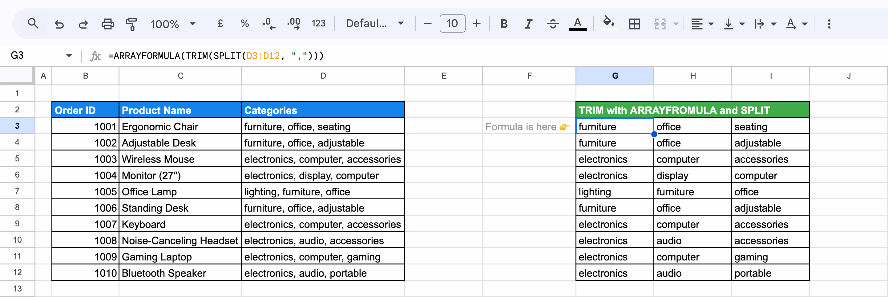
Suppose you have a dataset where multiple categories for each product are listed in a single cell, separated by commas. You can use ARRAYFORMULA, TRIM, and SPLIT to separate these categories into individual rows.
Use this formula:
=ARRAYFORMULA(TRIM(SPLIT(D3:D12, ",")))
Here:
- SPLIT(D3:D12, ","): The SPLIT function separates the categories in D3:D12 based on commas, dividing them into individual cells.
- TRIM(SPLIT(D3:D12, ",")): The TRIM function removes any leading or trailing spaces from the resulting text.
- ARRAYFORMULA: The ARRAYFORMULA allows the SPLIT and TRIM functions to be applied across the entire range, returning cleaner rows in a single step.
By combining ARRAYFORMULA, TRIM, and SPLIT, you can quickly clean and organize data in Google Sheets.
Joining ARRAYFORMULA, TRIM, FLATTEN, and SPLIT for Columns
Combining ARRAYFORMULA, TRIM, FLATTEN, and SPLIT functions in Google Sheets lets you clean and organize data efficiently. This method helps split values in a cell, remove extra spaces, and display the cleaned data in a single column for easier analysis.
Example:
Suppose you have a list of categories with multiple values that are separated by commas. Let's split these values into separate rows, remove extra spaces, and organize the data into a single clean column.
Use this formula:
=ARRAYFORMULA(TRIM(FLATTEN(SPLIT(D3:D5, ","))))

Here:
- SPLIT(D3:D5, ","): The SPLIT function separates the values in each cell from D3:D5, dividing them wherever a comma (,) appears. This breaks the text into separate pieces.
- FLATTEN(SPLIT(D3:D5, ",")): The FLATTEN function converts the array of values returned by SPLIT into a single column, stacking the values vertically.
- TRIM(FLATTEN(SPLIT(D3:D5, ","))): The TRIM function ensures that any leading or trailing spaces are removed from the split values, ensuring clean and consistent data.
- ARRAYFORMULA: The ARRAYFORMULA function allows the SPLIT, FLATTEN, and TRIM functions to be applied to the entire range processing multiple cells at once.
The formula will split, clean, and reorganize your data into a single column, removing any extra spaces and making the data easier for analysis or reporting.
Removing Extra Spaces with TRIM, REGEXREPLACE, and SUBSTITUTE
Removing extra spaces in data is crucial for ensuring consistency and readability. By combining the TRIM, REGEXREPLACE, and SUBSTITUTE functions in Google Sheets, you can efficiently clean up unwanted spaces, including non-breaking spaces and multiple consecutive spaces.
Example:
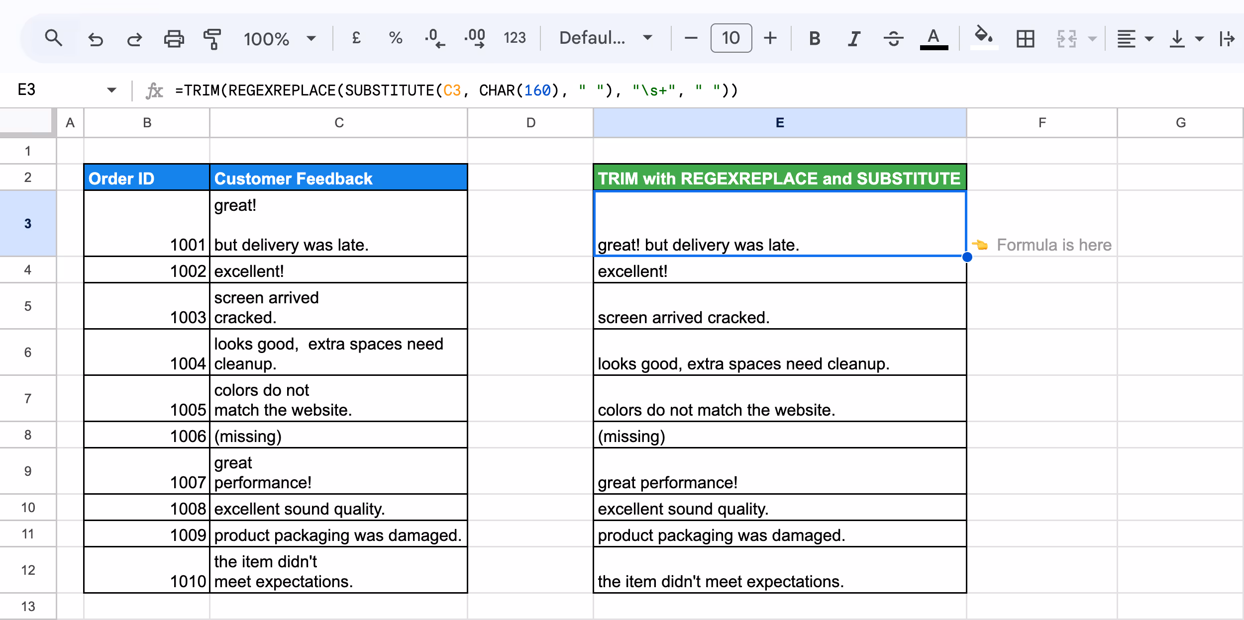
Suppose you have a Customer Feedback column where extra spaces or non-printable characters may exist. You can use the formula to clean the text, ensuring consistent formatting.
Use this formula:
=TRIM(REGEXREPLACE(SUBSTITUTE(C3, CHAR(160), " "), "\s+", " "))
Here:
- SUBSTITUTE(C3, CHAR(160), " "): Replaces non-breaking spaces (CHAR(160)) in the feedback with regular spaces.
- REGEXREPLACE(..., "\s+", " "): Replaces any sequence of multiple spaces with a single space.
- TRIM(...): Removes any leading or trailing spaces from the cleaned text.
By using TRIM, REGEXREPLACE, and SUBSTITUTE together, you can clean up Customer Feedback data by removing extra spaces and non-printable characters.
💡 Want to master REGEX functions in Google Sheets? Check out our detailed article to learn how to harness the power of regular expressions for more efficient data manipulation. Don't miss out on transforming your data skills! Read the full article here.
Combining TRIM and CONCATENATE to Clean and Merge Text
The TRIM and CONCATENATE functions in Google Sheets allows you to clean up text by removing unwanted spaces and then merge it into a single, neatly formatted string. This approach ensures that the resulting text is free of extra spaces and ready for further use or analysis.
Example:
Suppose you have product names with extra spaces between words, and you want to merge them into a single cell with the order ID . By combining TRIM and CONCATENATE, you can clean and merge text data in Google Sheets.
Use this formula:
=CONCATENATE(TRIM(B3), " ", TRIM(C3))
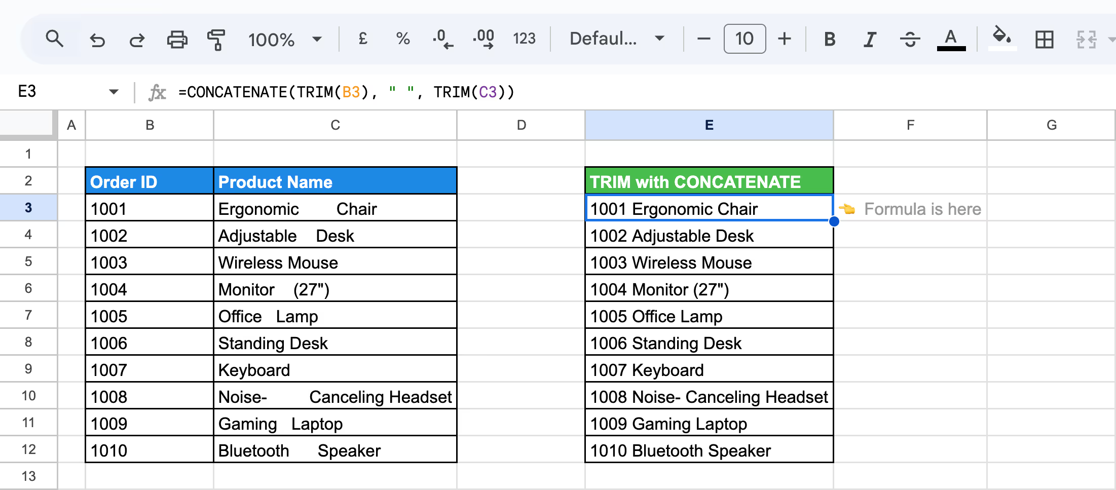
Here:
- TRIM(B3): Removes any leading, trailing, or extra spaces from the Order ID in B3.
- TRIM(C3): Similarly, removes any extra spaces from the Product Name in C3.
- CONCATENATE(TRIM(A2), " ", TRIM(B2)): Combines the cleaned text from B3 and C3, with a single space in between.
By combining TRIM and CONCATENATE, you can efficiently clean and merge text values, ensuring your data is tidy and ready for further analysis.
Combining CLEAN and TRIM Functions for Comprehensive Text Cleanup
Combining the CLEAN and TRIM functions provides a powerful way to clean up text data. This helps in removing any leading or trailing spaces from the text strings.
Example:
Suppose you have a Product Names column containing extra spaces and non-printable characters. You can clean and format the text in Google Sheets using the CLEAN and TRIM functions.
Use this Formula:
=(TRIM(CLEAN(C3:C12)))
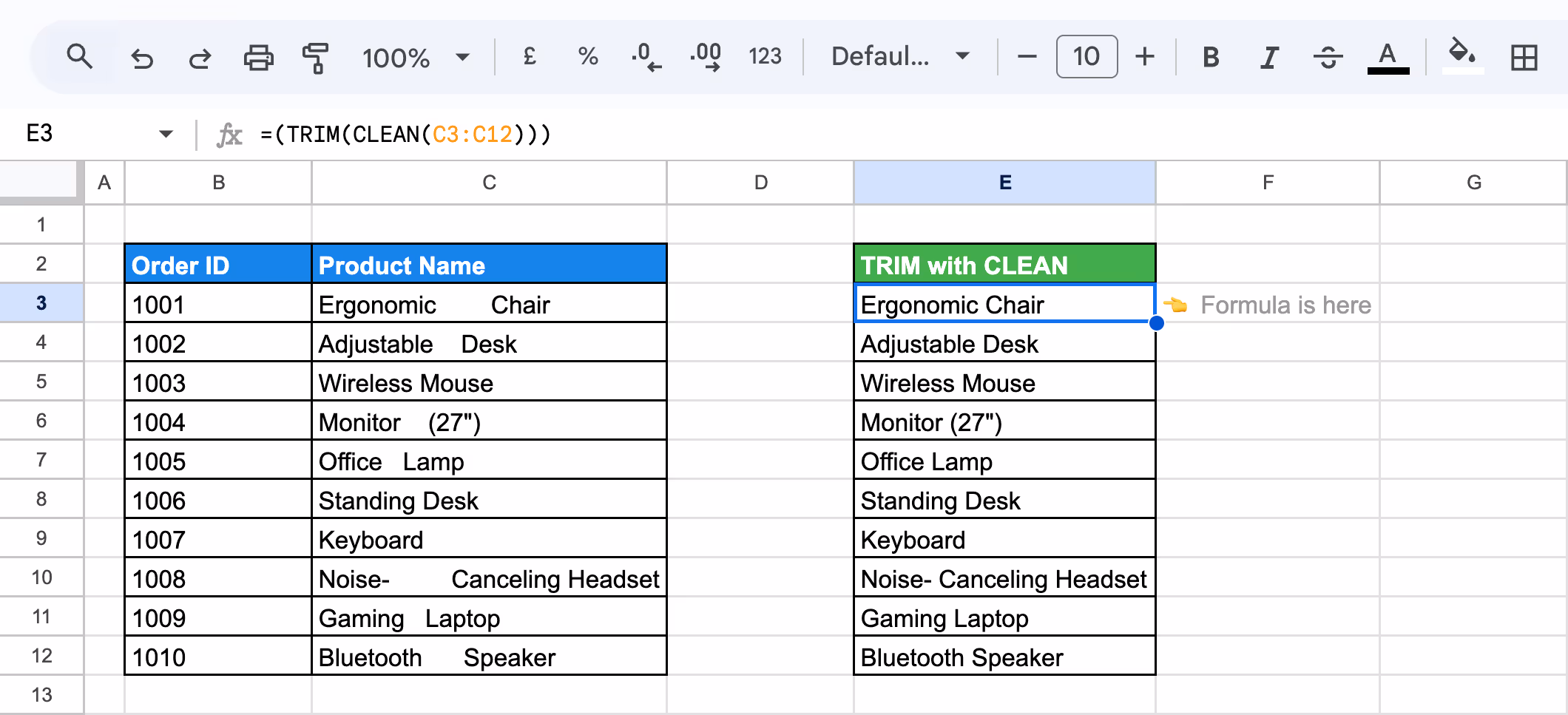
Here:
- CLEAN(C3:C12): The CLEAN function removes any non-printable characters from the Product Name column.
- TRIM(CLEAN(C3:C12)): The TRIM function removes any leading or trailing spaces from the cleaned text, ensuring consistent formatting.
Using the CLEAN and TRIM functions together allows you to remove unwanted characters and extra spaces from your text data.
Advanced Data Cleaning with CLEAN, TRIM, SUBSTITUTE, and PROPER
Advanced data cleaning in Google Sheets can be achieved by combining multiple functions like CLEAN, TRIM, SUBSTITUTE, and PROPER. These functions work together to remove unwanted characters, extra spaces, replace specific text, and ensure proper capitalization.
Example:
Suppose you have Customer Feedback data that contains unwanted spaces, non-printable characters, and inconsistent formatting (e.g., hyphens or capitalization issues). You can create a custom solution by combining these functions to clean and format the text properly.
Use this formula:
=PROPER(TRIM(CLEAN(SUBSTITUTE(C3, "-", " "))))
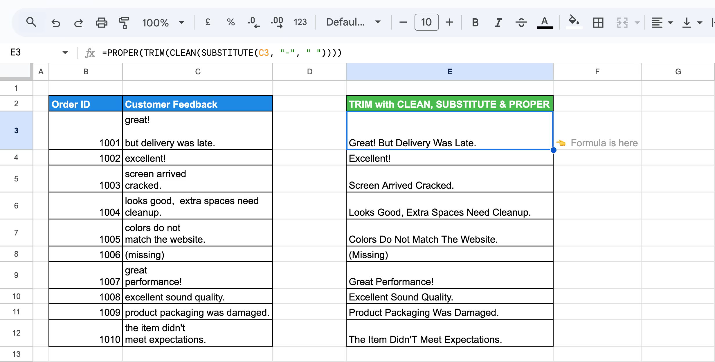
Here:
- SUBSTITUTE(C3, "-", " "): Replaces hyphens (-) with spaces in the Customer Feedback data in C3.
- CLEAN(C3): Removes any non-printable characters from the feedback.
- TRIM(CLEAN(...)): Removes any leading, trailing, or excessive spaces between words.
- PROPER(TRIM(...)): Capitalizes the first letter of each word, ensuring proper formatting.
By combining TRIM, CLEAN, SUBSTITUTE, and PROPER, you can create a powerful formula to clean and format your data in Google Sheets.
Combining T with CONCATENATE to Handle Mixed Data
When dealing with mixed data types in Google Sheets, the T function can be used to extract text values, while CONCATENATE helps combine those text values into one string. This approach ensures that only text values are considered, making it easier to handle and format mixed datasets effectively.
Example:
Suppose, with Order IDs (numeric) and Product Codes (alphanumeric). The goal is to concatenate these two columns, ensuring that both are treated as text and combined with a space in between.
Use this formula:
=CONCATENATE(T(B3), " ", T(C3))

Here:
- T(B3): Ensures that the Order ID (which is numeric) is treated as text.
- T(C3): Ensures that the Product Code (which may include both numbers and text) is treated as text.
- " ": Adds a space between the Order ID and Product Code.
- CONCATENATE: Combines the two text values (Order ID and Product Code) into one string.
The formula ensures that both values are treated as text and concatenated with a space in between, making it useful for joining product codes and names or any other text-based data.
Using T Function with IF for Text Detection
The T function in Google Sheets ensures that data is treated as text, even if it includes numbers or non-text values. By combining it with the IF function, you can create conditions that check for the presence of text in a cell. This method is useful for detecting whether a specific cell contains text or is empty, allowing for conditional actions based on that result.
Example:
Suppose you have a dataset with Order ID and Raw Data, and you want to identify whether the Raw Data column contains any text. This formula checks if there’s any content in the Raw Data field.
Use this formula:
=IF(LEN(T(C3))>0, "Text Present", "No Text")
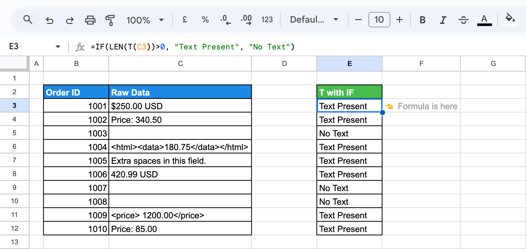
Here:
- T(C3): Ensures that the value in Raw Data (C3) is treated as text, even if it contains numbers or HTML tags.
- LEN(T(C3)) > 0: Checks if the length of the text in Raw Data (C3) is greater than zero (i.e., there is text in the field).
- "Text Present": If there is text, the formula returns "Text Present".
- "No Text": If the cell is empty or contains no text, it returns "No Text".
This formula is useful for quickly identifying rows with missing or empty data, allowing for easier data validation and cleanup.
Highlighting Text with Conditional Formatting Using LEN and T Function
Using LEN and the T function in conditional formatting allows you to highlight cells that contain text, even if they include special characters or numbers. This method helps visually identify text entries in a dataset, making it easier to spot and organize relevant information.
Example:
Suppose you have the following Raw Data and want to highlight cells that contain text, including those with special characters, numbers, or embedded HTML tags.
But before applying the formula, you need to set up the Conditional Formatting:
- Select the range of cells where you want to apply conditional formatting (e.g., C3:C12).
- Go to Format → Conditional formatting.
- Under the Format cells if dropdown, choose Custom formula is.
Use this formula:
=LEN(T(C3))>0
- Set your desired formatting style (e.g., background color or text color).
- Click Done.

Here:
- T(C3): will convert the value in the cell to text (including any numbers or special characters).
- LEN(T(C3)): checks the length of the text in the cell.
- >0: ensures that the formula only highlights cells that have text (i.e., any non-empty cell will be formatted).
Using LEN and T in conditional formatting ensures that all cells containing text are highlighted, which helps you easily identify and visually organize text-based data in your dataset.
Troubleshooting Common Issues with TRIM, CLEAN, and T Functions
In this section, we'll address troubleshooting common issues with the TRIM, CLEAN, and T functions in Google Sheets. These functions are powerful tools for data management but can sometimes lead to unexpected results if not used correctly. We will explore common pitfalls such as handling special character types, updating cell references, and the correct usage of these functions with different data types.
Missing Non-breaking Spaces
⚠️ Error: The TRIM function does not remove non-breaking spaces, which can cause issues when cleaning data. These spaces are often invisible but still affect text formatting and comparisons.
✅ Solution: If TRIM isn't removing the unwanted spaces, implement a more comprehensive cleaning strategy. Replace non-breaking spaces with regular spaces using a suitable function, then apply TRIM to clean the text. This ensures that all spaces, including non-breaking ones, are removed.
Failing to Update Cell References
⚠️ Error: If you move or alter your data, make sure you update your TRIM and T function references. Otherwise, you might trim the wrong cells or columns, leading to inaccurate results.
✅ Solution: Ensure your TRIM and T functions reference the correct cells or values. After moving or altering your data, double-check and update the cell references in your formulas to avoid trimming incorrect data or leaving references empty.
Misusing TRIM and T on Numeric Data
⚠️ Error: TRIM is explicitly designed for text, so applying it to numeric data could inadvertently convert the numbers into text. This can interfere with calculations and lead to errors. Similarly, the T function is intended for text values, and if used on numeric data, it will return an empty string, providing no sound output.
✅ Solution: Avoid using TRIM and T on purely numeric data. If your data is numeric, skip TRIM to prevent it from being converted to text. For the T function, ensure you only apply it to text values to get meaningful results.
Removing Non-ASCII Characters with CLEAN
⚠️ Error: The CLEAN function only removes ASCII codes 0-31 and 127 from the text string, which includes control characters but not punctuation or other non-printing characters. This means it won't clean all unwanted characters from your data.
✅ Solution: To remove punctuation, non-printing characters, or other unwanted symbols, use the SUBSTITUTE function in combination with CLEAN. To clean the text thoroughly, you can replace specific characters with an empty string.
CLEAN Function Does Not Modify or Transform Text
⚠️ Error: The CLEAN function requires the text argument to be a text string or a reference to a cell containing a text string. Using a formula, expression, or a non-text value (like a number or date) as the text argument will result in an error.
✅ Solution: Ensure that the argument passed to the CLEAN function is either a valid text string or a cell reference that contains text. If you need to clean numeric or date values, convert them to text using the TEXT function before applying CLEAN.
T Function Does Not Convert Numbers to Text
⚠️ Error: The T function does not convert numbers to text. It strictly checks if the value is text, and if so, returns the text. If the value is not text (including numbers or other non-text values), it returns an empty string.
✅ Solution: Ensure you only use the T function when checking for text values. If you need to convert numbers to text, use the TEXT function instead, as it can format numbers as text based on the specified format.
Best Practices for Using TRIM, CLEAN, and T Functions
When managing text in Google Sheets, applying functions correctly is crucial for keeping your data clean and precise. This section outlines best practices for using the TRIM, CLEAN, and T functions effectively, which will help you improve your data management techniques.
Build a Reusable Cleaning Template
Create a Google Sheets template with the TRIM function applied to columns you regularly clean. This approach streamlines your workflow, saves time, and ensures consistent formatting across different datasets.
Use LEN to Verify Cleaned Data
Apply the LEN function before and after using TRIM to check if spaces have been successfully removed. This quick verification ensures that your data has been cleaned properly, giving you confidence in the results.
Using Google Apps Script
Leverage Google Apps Script to automate the application of the TRIM function across large datasets. By writing a custom script, you can efficiently clean multiple ranges or sheets with a single click, saving time on repetitive tasks.
Implementing Systematic Data Management Strategies
Maintain detailed documentation of your cleaning processes and establish a systematic approach to data cleaning. Include regular validation checks to ensure accuracy. This practice promotes consistency across spreadsheets and makes it easier for others to understand your methodology.
Optimizing Performance for Large Datasets with Array Formulas
Consider using array formulas to process multiple cells at once when handling large datasets. With helper columns, break down complex cleaning tasks into smaller steps. This approach improves formula readability, enhances efficiency, and simplifies troubleshooting.
Combining with Other Functions for Advanced Text Patterns
Improve text manipulation by effectively utilizing the T function in combination with other functions like ARRAYFORMULA. This technique allows you to apply the T function across a range without manually extending the formula. It ensures that operations are only applied to text data, making your data handling more complex and dynamic.
Use Conditional Formatting
After using the TRIM function to clean up leading or trailing spaces, employ conditional formatting to identify cells still containing spaces. Additionally, utilize the T function in conditional formatting to selectively highlight text values, making it easier to recognize patterns in your data. This method ensures your data remains organized and enhances visual tracking, improving both data cleanliness and analysis.
Create Dynamic Ranges
Use the T function to create ranges that include only text values dynamically. This is particularly useful for filtering data for charts or analysis, ensuring that only relevant text entries are included, and improving the accuracy and focus of your data visualizations.
Essential Google Sheets Functions for Advanced Data Analysis
Google Sheets offers a wide variety of powerful functions that simplify data analysis, enabling users to easily handle and interpret large datasets. These essential functions help you extract insights, manage data efficiently, and perform in-depth analysis with minimal effort.
- UNIQUE: Extracts unique values from a range, removing duplicates to give you a cleaner dataset.
- IMPORTRANGE: Imports a specific range of cells from another spreadsheet, making consolidating data across multiple sheets easy.
- MATCH: Searches for a value within a range and returns the relative position of that value, aiding in lookups and data comparison.
- COUNTA: Counts the number of non-empty cells in a range, useful for tracking data presence or tallying entries.
- MAX, MIN, MEDIAN: These functions allow you to find the highest value (MAX), the lowest value (MIN), or the middle value (MEDIAN) in a dataset, essential for summary statistics.
- TIME: Converts hours, minutes, and seconds into a time value, simplifying time-based calculations.
- WORKDAY: Calculates a date that is a specified number of working days (excluding weekends and holidays) from a given date.
- ROUND: Rounds a number to a specified number of digits, useful for formatting and presenting data consistently.
Visualize Your Data with OWOX: Reports, Charts, and Pivot Tables
Using TRIM, CLEAN, and T functions can help tidy your data, but automating the entire process can save you even more time. OWOX Reports takes your data cleaning to the next level with automated reports, dynamic charts, and seamless data imports.
Whether you're removing excess spaces or organizing text, OWOX simplifies the process so you can focus on insights. Install the OWOX Reports today and make your data workflow faster and smarter!
Frequently asked questions


Finally, a tool that doesn't ask business users to learn a new dashboarding UI. Our marketing team already knows Sheets. OWOX just delivers the right data.
Joinable data marts concept was the thing that sold us. We can now use the semantic layer without building one.
Self-hosted the OSS version on Digital Ocean. Zero vendor lock-in. Contributed a Shopify connector back in week two.