
Effortless Text Combination in Google Sheets with & and CONCATENATE Function
Master Google Sheets functions like AMPERSAND and CONCATENATE. Practical tips for merging text, using separators, and generating dynamic content.


Are you looking to enhance your spreadsheets by combining text seamlessly? Google Sheets offers two powerful tools for this purpose: the ampersand (&) and the CONCATENATE function.
These methods simplify the process of merging text strings, crucial for refining report presentation, organizing data efficiently, or automating routine spreadsheet tasks.
This guide delves into the practical applications of both tools, demonstrating how to use them to create cleaner, more effective spreadsheets. Explore the steps to seamlessly integrate text in Google Sheets, boosting your productivity and bringing greater functionality to your data management practices.
Advantages of Using CONCATENATE and AMPERSAND in Google Sheets
Using CONCATENATE and the AMPERSAND operator in Google Sheets offers several benefits:
- Improved Data Organization: Effortlessly combine text values, such as names and addresses, into single fields for better accessibility.
- Time Savings: Avoid manual entry by merging data from multiple columns automatically.
- Enhanced Readability: Include separators (e.g., commas, spaces) for clean, structured outputs.
- Streamlined Workflow: Create reusable, dynamic formulas for tasks like generating summaries or personalized data presentations.
- Custom Data Presentation: Tailor data for reports or templates by merging text based on specific conditions.
These features make CONCATENATE and the AMPERSAND operator essential tools for efficient and flexible text management in Google Sheets.
Using CONCATENATE and AMPERSAND: Syntax and Detailed Examples
The CONCATENATE function and the AMPERSAND (&) operator in Google Sheets allow users to merge text, numbers, and dates from multiple cells into one. By combining these tools with separators, formulas, or conditions, you can create dynamic outputs such as labels, summaries, or custom reports, simplifying data organization and enhancing efficiency.
CONCATENATE Function
The CONCATENATE function in Google Sheets combines text, numbers, or dates from multiple cells into a single cell. It's a powerful tool for merging data, creating labels, or formatting outputs. By using CONCATENATE with separators like commas or spaces, you can organize information efficiently and enhance readability in your spreadsheets.
Syntax of CONCATENATE
The CONCATENATE function in Google Sheets allows you to join multiple text strings, numbers, or cell references into a single string.
The syntax for the function is:
=CONCATENATE(string1, [string2, ...])
The date argument can be provided in several ways, including:
- string1 (required): The first text string, number, or cell reference to be combined.
- string2, string3, ... (optional): Additional text strings, numbers, or cell references to combine with the first one.
You can also include spaces, commas, or other characters as separators by wrapping them in quotation marks (e.g., " " or ", ") and listing them as arguments. This function is ideal for creating labels, combining fields, or formatting data for reports, offering a simple yet powerful way to manage text in spreadsheets.
Example of CONCATENATE
Imagine you have a dataset containing first names, last names, and salaries. You want to create a new column that displays the full name along with the salary in a formatted sentence, such as “John Doe earns $55,000.”
To achieve this, use the formula:
=CONCATENATE(B3, " ", C3, " earns $", D3)
Here’s the breakdown:
- CONCATENATE: Joins multiple text strings or cell values into a single string.
- B3: Refers to the first name
- " ": Adds a space between the first and last name.
- C3: Refers to the last name.
- " earns $": Adds the descriptive text before the salary.
- D3: Refers to the salary value.

This example demonstrates how CONCATENATE simplifies the process of creating meaningful and formatted outputs from your data.
Ampersand (&) Operator
The Ampersand (&) operator in Google Sheets provides a straightforward way to join text, numbers, or cell values. It allows for the seamless combination of multiple elements into a single string, making it a versatile and efficient tool for organizing and presenting data in spreadsheets. Its simplicity makes it accessible for users of all skill levels.
Syntax of Ampersand (&)
The Ampersand (&) operator in Google Sheets is used to join text, numbers, or cell values into a single string.
Its syntax is straightforward:
=value1 & value2 [& value3, ...]
The function requires arguments:
- value1, value2, ...: Represent the elements being combined, which can include text, numbers, or cell references.
- separators: Spaces, commas, or other characters can be added as text strings enclosed in quotation marks (e.g., " " or ", ") between values.
This operator offers flexibility for combining various data types while keeping formulas simple and intuitive.
Example of Ampersand (&)
The Ampersand (&) operator is a quick and efficient way to combine text and numbers in Google Sheets. Using the demo dataset, let’s create a sentence that includes an employee's full name and department. For example, "John Doe works in Marketing."
Let's use the formula:
=B3 & " " & C3 & " works in " & D3
Here’s the breakdown:
- &: The concatenation operator that combines text and cell values.
- B3: Refers to the first name.
- " ": Adds a space between the first and last name.
- C3: Refers to the last name.
- " works in ": Adds descriptive text before the department name.
- D3: Refers to the department name.
.avif)
Why this method is useful:
- Simple Syntax: The Ampersand makes combining values straightforward without the need for a specific function.
- Flexible Formatting: Add spaces, punctuation, or other characters for clarity.
- Dynamic Updates: The combined output automatically updates when source values change.
This example highlights how the Ampersand operator simplifies text merging tasks in spreadsheets.

Basic Examples of Using CONCATENATE and Ampersand in Google Sheets
CONCATENATE and the Ampersand operator are essential tools for combining text, numbers, and cell values efficiently. These functions allow you to format data dynamically, merge columns, and create clean, readable outputs. Whether adding separators or generating labels, both methods simplify text handling in Google Sheets.
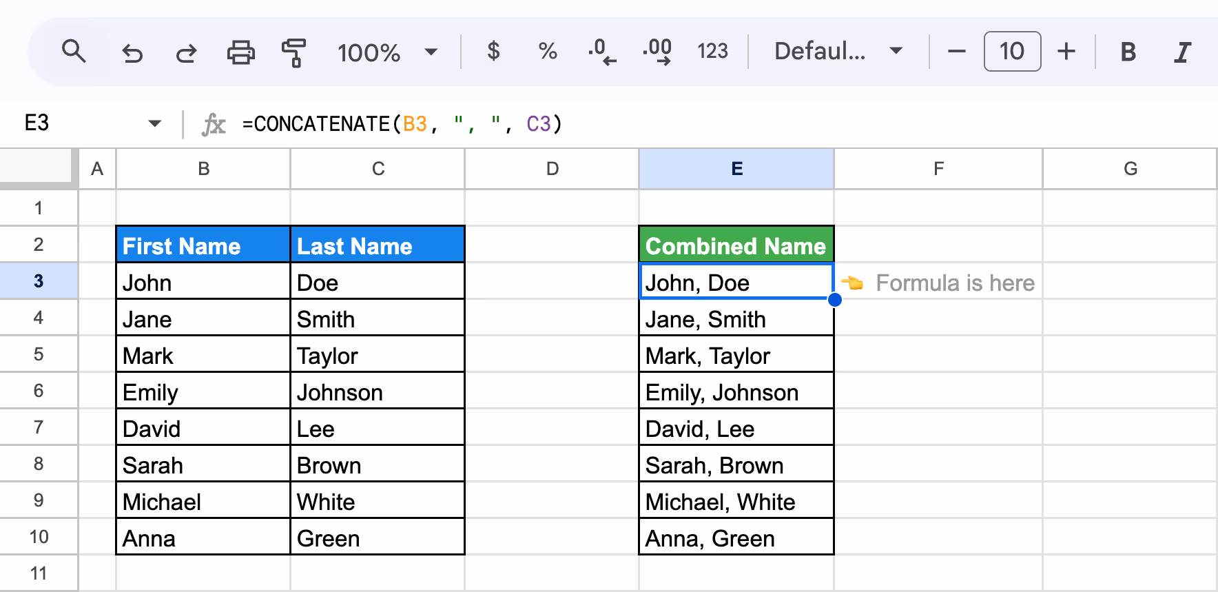
Using CONCATENATE to Separate Values with a Comma Separator
The CONCATENATE function in Google Sheets can efficiently combine values while adding separators like commas to organize data. This is particularly useful for creating lists or structured outputs, such as combining names and locations for reports.
To combine first and last names with a comma and space separator, use the formula:
=CONCATENATE(B3, ", ", C3)
Here’s the breakdown:
- B3: Refers to the first name.
- ", ": Adds a comma and space as the separator.
- C3: Refers to the last name.
- CONCATENATE: Joins cell values into one continuous string.
By using the function CONCATENATE, you can organize data cleanly and ensure consistency across your spreadsheets. It’s a practical solution for managing large datasets efficiently and presenting information professionally.
Combining Two Columns Using CONCATENATE
Combining two columns in Google Sheets using the CONCATENATE function allows users to merge values efficiently without additional separators. This method is perfect for situations where you need to create identifiers, join raw data, or merge text fields directly.
To combine two columns without a separator, use the formula:
=CONCATENATE(B3, C3)
Here’s the breakdown:
- B3: The first column (e.g., First Name).
- C3: The second column (e.g., Last Name).
- CONCATENATE: The function joins cell values into one continuous string.
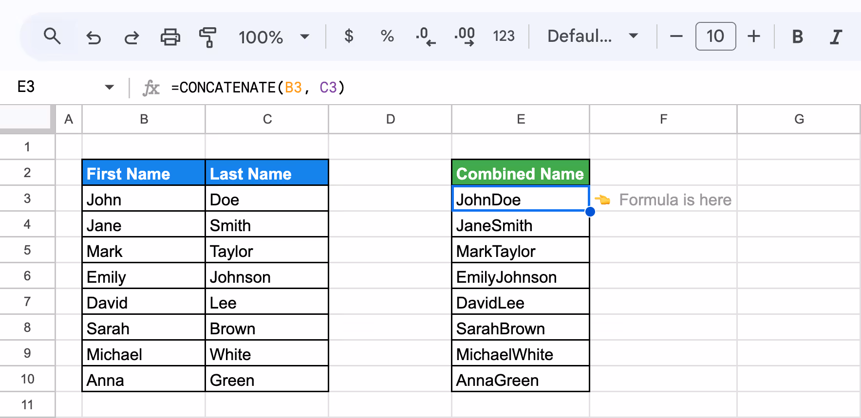
This approach highlights how CONCATENATE simplifies data merging tasks, making it an essential tool for managing spreadsheet data efficiently.
Applying CONCATENATE to Multiple Rows
Using the CONCATENATE function to combine values from multiple rows in Google Sheets allows you to merge data into a single cell, creating summaries, combined labels, or reports. Google Sheets offers multiple ways to apply the CONCATENATE function across multiple rows, saving time and reducing manual work:
1. Drag to Autofill:
Select the cell containing your CONCATENATE formula. Click on the small square (fill handle) at the bottom-right corner of the cell, then drag it down to apply the function to additional rows. This method works well for consistent patterns.
2. Autofill with Suggested Formula:
After entering the CONCATENATE formula in one cell, Google Sheets may automatically trigger an autofill suggestion for the remaining rows. Simply click the checkmark to confirm and apply the formula across all rows.
Why these methods are useful:
- Efficiency: Saves time when working with large datasets.
- Flexibility: Adapts to various scenarios, from specific rows to entire columns.
- Accuracy: Reduces manual errors when applying formulas across multiple rows.
By leveraging these techniques, users can streamline text combination processes and manage data effectively in Google Sheets.
Using CONCATENATE to Create Financial Budget Labels
The CONCATENATE function can be combined with the TEXT function to format numeric values, such as salaries or budgets, with commas for better readability. This approach is ideal for creating clear, professional financial labels.
To create labels with properly formatted numbers, use:
=CONCATENATE("Q1 Budget: $", TEXT(B3, "#,##0"))
Here’s the breakdown:
- "Q1 Budget: $": Adds a descriptive text label and a dollar sign.
- C3: Refers to the numeric value.
- TEXT(C3, "#,##0"): Formats the number with commas for thousands separators.

Why This is Useful:
- Formatted Outputs: Combines text with numbers, formatted for clarity.
- Professional Reporting: Makes financial data easier to read and present.
- Dynamic and Flexible: Updates automatically when the source data changes.
This method ensures that budget labels are well-structured, visually clear, and ready for professional use.
Basic Use of the Ampersand Operator for Joining Text
The Ampersand (&) operator in Google Sheets is a simple yet powerful tool for combining text, numbers, or cell values. It works by connecting multiple elements into a single string without requiring a dedicated function. This is especially useful for adding prefixes, suffixes, or merging fields dynamically.
To combine two cells with a space in between, use:
=B3 & " " & C3
Here’s the breakdown:
- B3: Refers to the value in cell B3.
- &: The concatenation operator that combines values and text.
- " ": Adds a space between the two values for proper formatting.
- C3: Refers to the value in cell C3.
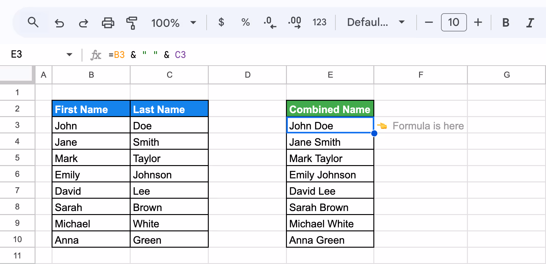
This method is ideal for generating full names, creating dynamic labels, and combining text efficiently, ensuring a smooth and user-friendly experience.
Advanced Examples of Using CONCATENATE and Ampersand in Google Sheets
Beyond basic text merging, CONCATENATE and the Ampersand operator allow for advanced data manipulation. These methods can combine multiple columns, add separators, format dates, and create unique identifiers. By incorporating these techniques, users can generate detailed, dynamic, and professional outputs tailored to various reporting and organizational needs.
Combining Multiple Columns with CONCATENATE
The CONCATENATE function in Google Sheets can be used to merge multiple columns while adding separators like commas for better clarity. This is particularly useful for creating structured data outputs, such as lists or summaries, from separate columns.
Let's use the formula:
=CONCATENATE(B3, ", ", C3, ", ", D3)
Here’s the breakdown:
- B3: Refers to the First Name.
- ", ": Adds a comma and space separator between values.
- C3: Refers to the Department.
- D3: Refers to the Salary column.
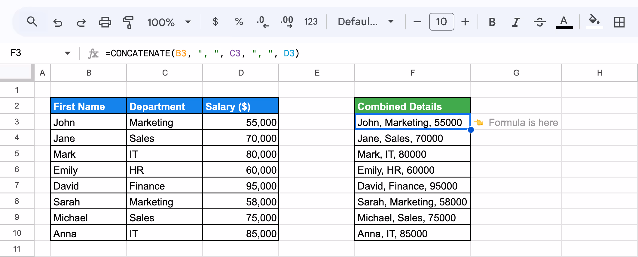
This method demonstrates how CONCATENATE efficiently combines multiple fields into a clear and concise output, perfect for reports and data summaries.
Using CONCATENATE with Separators for Detailed Information
The CONCATENATE function in Google Sheets can include separators like commas, spaces, or dashes to organize and format combined information. This method is ideal for creating structured data outputs such as employee summaries, addresses, or labels.
To combine First Name, Department, and Salary with separators for readability, use:
=CONCATENATE(B3, " - ", C3, " | $", D3)
Here’s the breakdown:
- B3: Refers to the First Name.
- " - ": Adds a dash to separate fields.
- C3: Refers to the Department.
- " | $": Adds a pipe and dollar sign for clarity.
- D3: Refers to the Salary column.
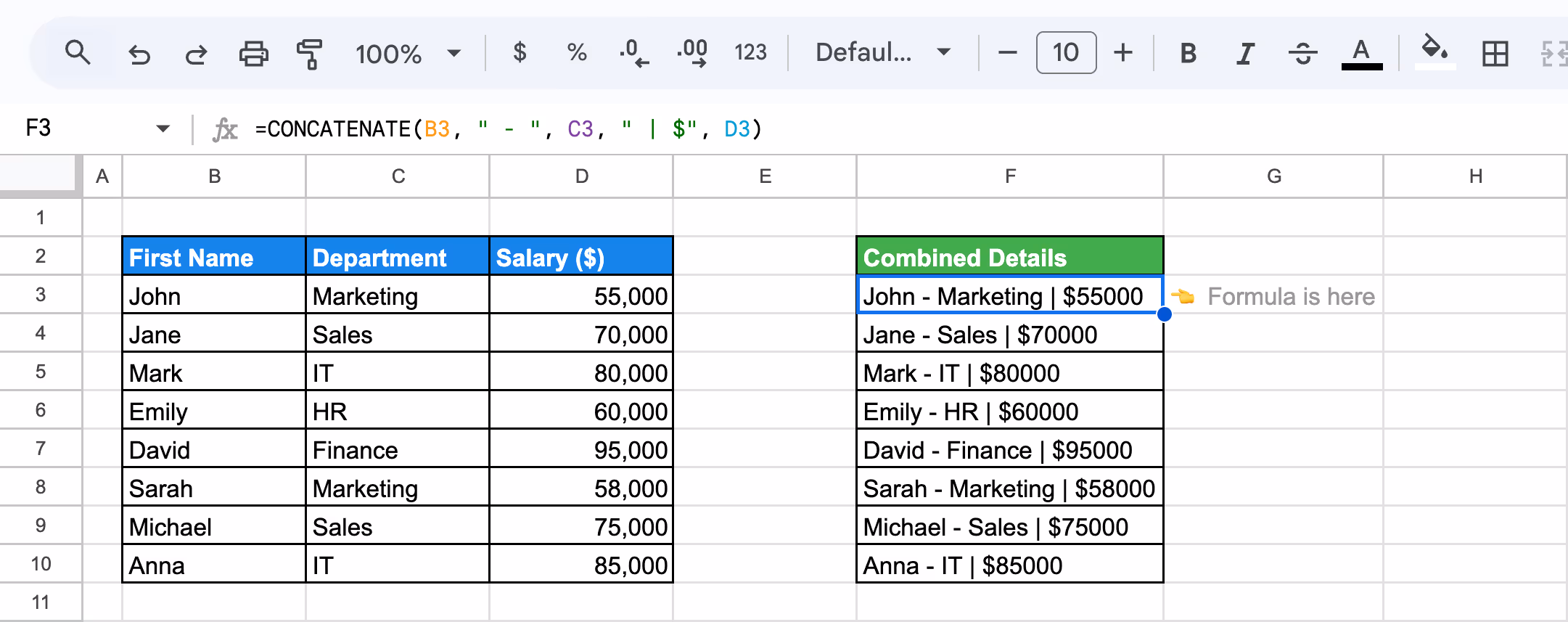
This method highlights how CONCATENATE, with separators, transforms raw data into polished and professional summaries.
Concatenating Text from Multiple Cells with Space Using Ampersand
The Ampersand (&) operator is a quick and flexible way to combine text from multiple cells with spaces in between. Unlike the CONCATENATE function, the Ampersand requires minimal syntax and works efficiently for merging values in a readable format.
To combine information from cells with spaces in between, use the formula:
=B3 & " " & C3 & " " & D3
Here’s the breakdown:
- B3: Refers to the value in cell B3.
- &: The concatenation operator that combines values and text.
- " ": Adds a single space between the values for proper formatting.
- C3: Refers to the value in cell C3.
- D3: Refers to the value in cell D3.
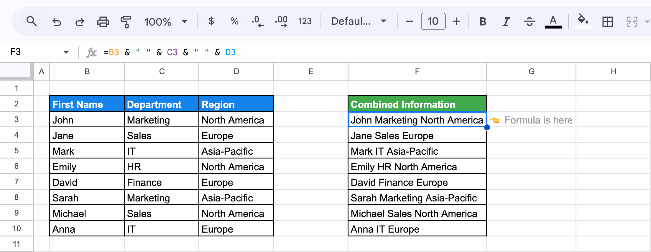
This method is perfect for combining text across multiple cells efficiently while maintaining clarity in your data presentation.
Concatenating Dates into Informative Entries
In Google Sheets, the CONCATENATE function or the Ampersand (&) operator can merge text with dates to create informative entries. Using the TEXT function alongside CONCATENATE ensures that dates are displayed in a readable format.
Let's use the formula:
=CONCATENATE(B3, " joined on ", TEXT(C3, "mmmm dd, yyyy"))
Here’s the breakdown:
- B3: Refers to the First Name.
- " joined on ": Adds contextual text for clarity.
- TEXT(C3, "mmmm dd, yyyy"): Formats the date in a full month, day, and year style.
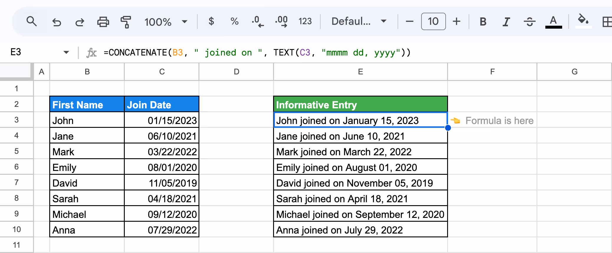
This method is perfect for creating reports, logs, or timelines that combine text with formatted dates efficiently.
Concatenating Numbers for Unique Identifiers
The CONCATENATE function in Google Sheets can merge numbers or text with separators to generate unique identifiers or reference codes. This is particularly useful for combining product codes, employee IDs, or tracking numbers into a single field for clarity and organization.
The formula will be:
=CONCATENATE(B3, "-", C3)
Here’s the breakdown:
- B3: Refers to the First Name.
- "-": Adds a hyphen as a separator.
- C3: Refers to the numeric Target (%) value.
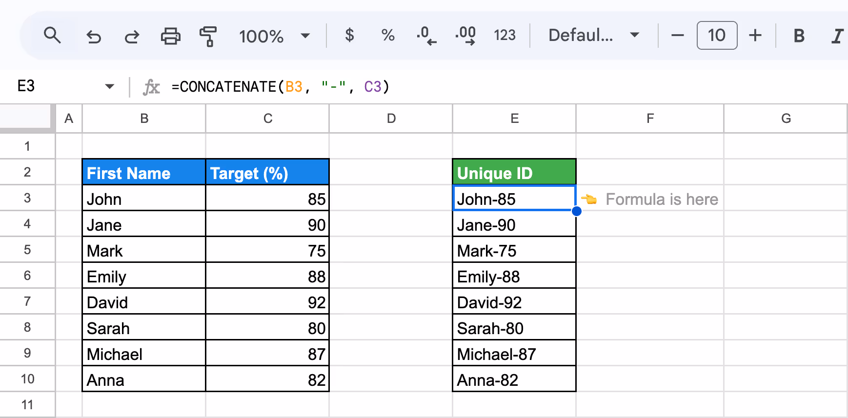
This method efficiently merges data fields to produce clear and professional unique identifiers, simplifying organization and reporting tasks.
Merging Text and Dates Using Ampersand
The Ampersand (&) operator in Google Sheets makes it easy to merge text with dates. However, to display dates in a readable format, you need to use the TEXT function. This method is perfect for creating logs, timelines, or summaries with dynamic text and dates.
Let's use the formula:
=B3 & " joined on " & TEXT(C3, "mm/dd/yyyy")
Here’s the breakdown:
- B3: Refers to the First Name.
- " joined on ": Adds contextual text.
- TEXT(C3, "mm/dd/yyyy"): Formats the date in a readable "month/day/year" format.
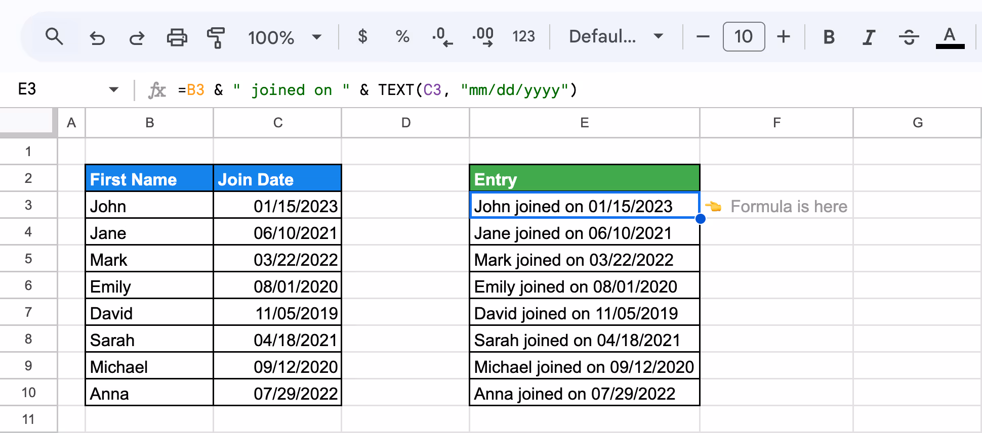
This approach is particularly useful for generating structured logs, event timelines, or reports where combining descriptive text with precise dates enhances readability and organization. It leverages the simplicity of the Ampersand operator while ensuring polished, professional outputs.
Combining CONCATENATE and Ampersand with Other Google Sheet Functions
By combining CONCATENATE and the Ampersand operator with other Google Sheets functions, you can create dynamic, automated outputs tailored to various use cases. These combinations enable advanced text formatting, conditional logic, date handling, and numeric calculations, enhancing your ability to manage and present complex datasets efficiently.
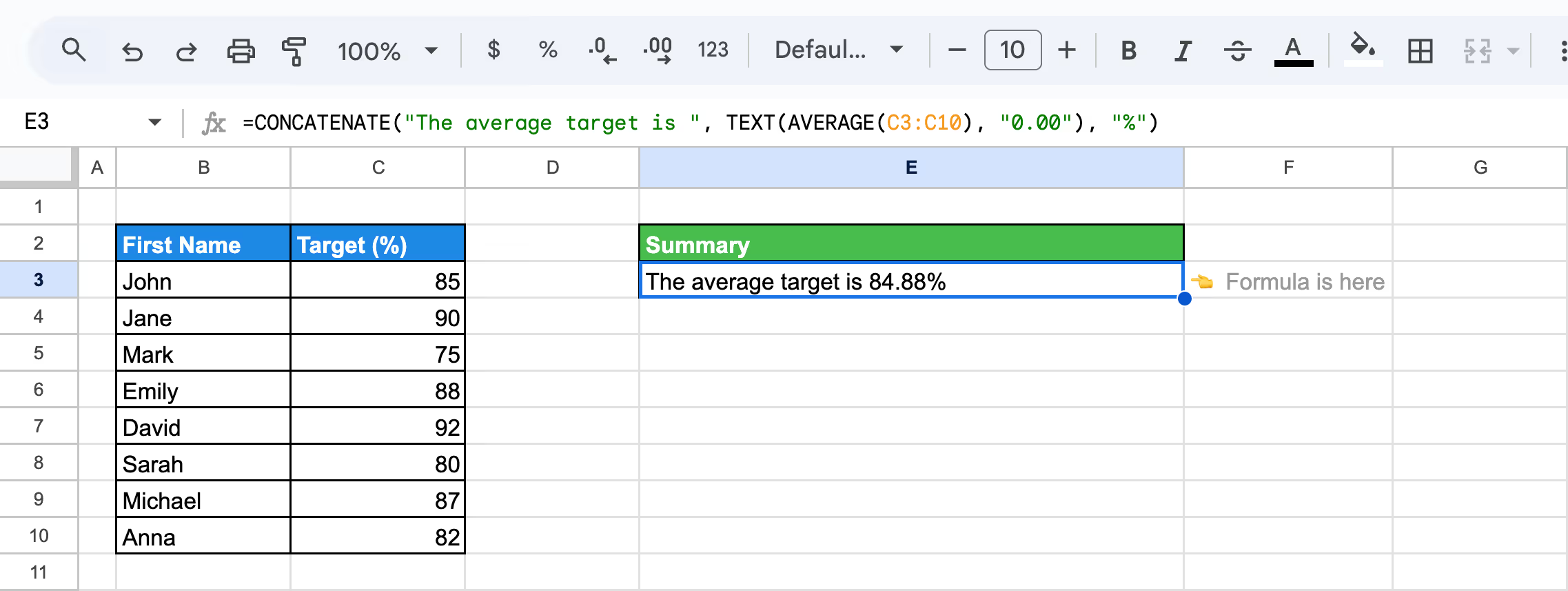
Combining Text Using CONCATENATE with TEXT and AVERAGE Functions
The CONCATENATE function can be combined with the TEXT and AVERAGE functions to display dynamic, readable summaries that include calculated values. This approach is ideal for generating formatted outputs that combine text and numeric results, such as average scores, financial summaries, or custom reports.
To create a summary that displays the average Target (%) with descriptive text, use the formula:
=CONCATENATE("The average target is ", TEXT(AVERAGE(C3:C10), "0.00"), "%")
Here’s the breakdown:
- AVERAGE(C3:C10): Calculates the average value of the Target column.
- TEXT(AVERAGE(...), "0.00"): Formats the result to display two decimal places.
- "The average target is ": Adds context to the output.
But if you want to combine a date and the calculated average Target (%) into a single formatted entry, use:
=CONCATENATE("As of ", TEXT(TODAY(), "MMMM dd, yyyy"), ", the average target is ", TEXT(AVERAGE(C3:C10), "0.0"), "%")
Here’s the breakdown:
- TEXT(TODAY(), "MMMM dd, yyyy"): Inserts today's date in a readable format.
- AVERAGE(C3:C10): Calculates the average target percentage.
- TEXT(..., "0.0"): Formats the average to one decimal place.
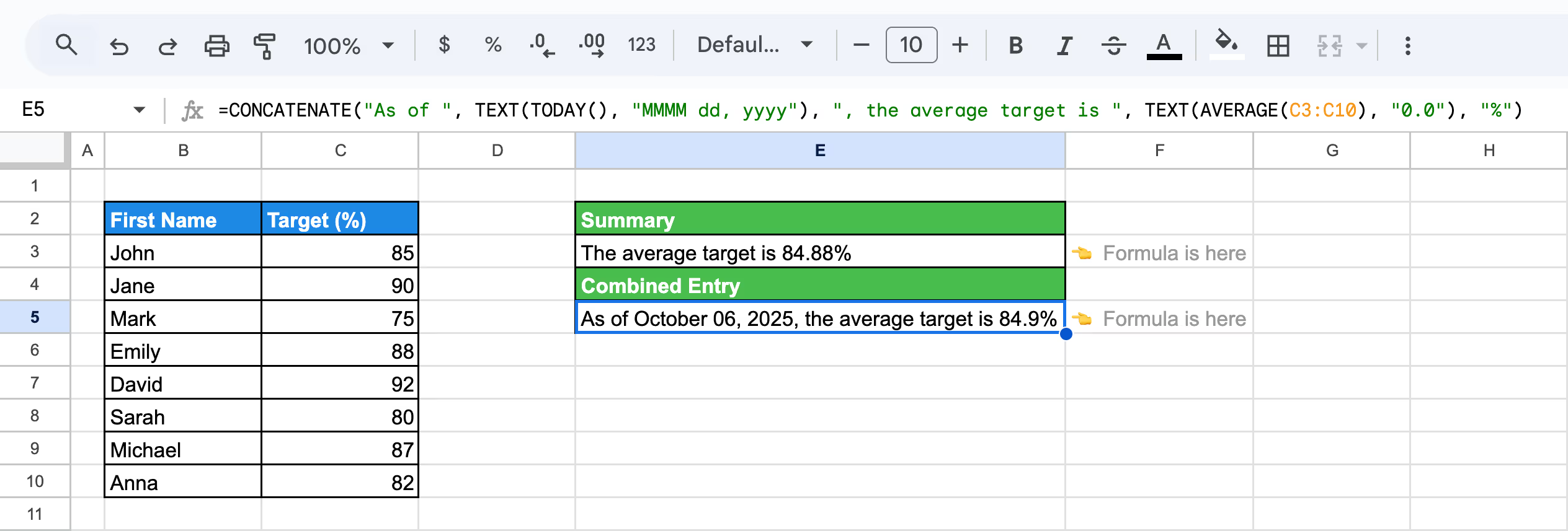
These variations showcase how CONCATENATE can be enhanced with TEXT and AVERAGE functions to create polished, dynamic summaries in Google Sheets.
Combining Text with Conditional Logic Using CONCATENATE and IF
The CONCATENATE function, combined with the IF function, allows for conditional text outputs based on specific criteria in your dataset. This approach is ideal for creating dynamic messages, such as performance summaries or status updates, based on cell values.
Let's use the formula:
=CONCATENATE(B3, " has ", IF(C3>=85, "met or exceeded", "not met"), " their target.")
Here’s the breakdown:
- B3: Refers to the First Name.
- " has ": Adds static text to the result.
- IF(С3>=85, "met or exceeded", "not met"): Checks if the Target (%) in С3 is greater than or equal to 85 and outputs the appropriate message.
- " their target.": Completes the statement.
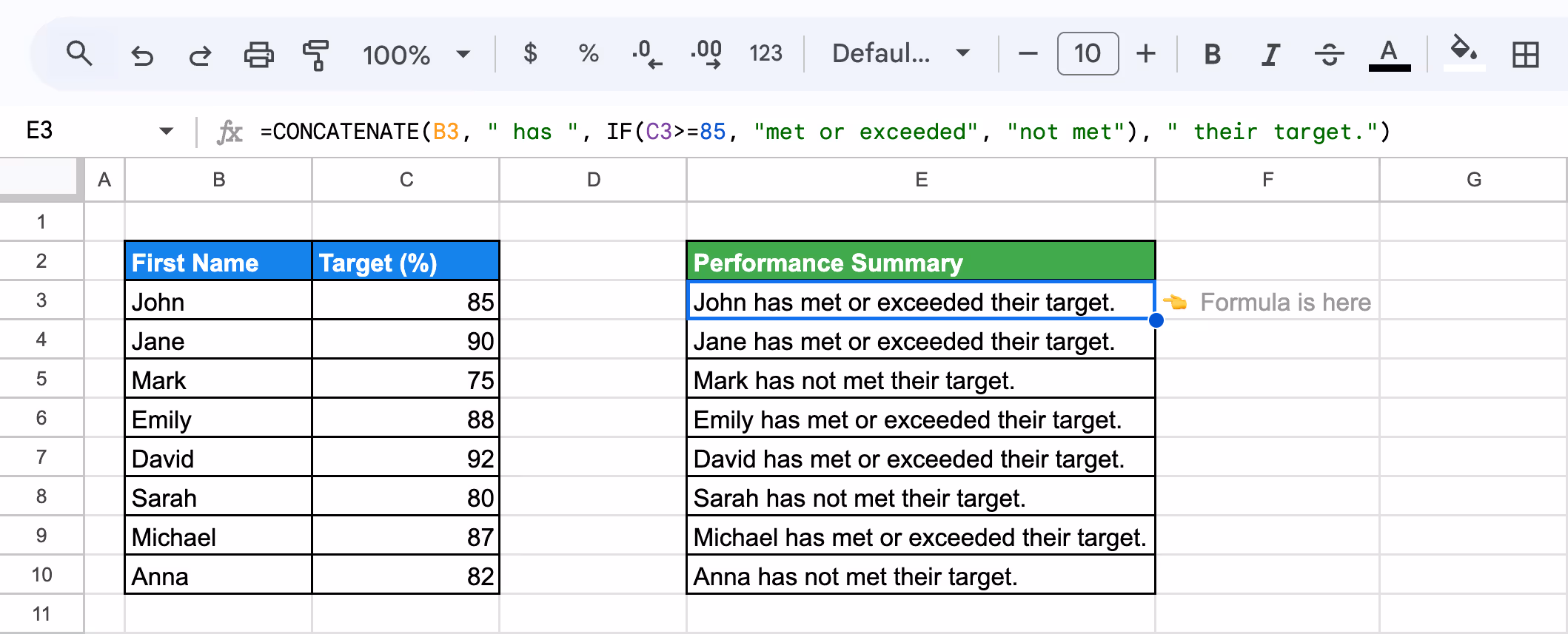
This method enhances reporting by combining logic and text to generate dynamic, actionable insights.
Using CONCATENATE with QUERY via TRANSPOSE Workaround
In Google Sheets, the combination of QUERY, TRANSPOSE, and CONCATENATE allows you to summarize filtered data into a single output. This method is particularly useful for merging specific rows based on conditions, such as listing employees in the "IT" department along with their projects.
To extract unique rows and transpose them for a compact view, use a formula like:
=TRANSPOSE(QUERY(TRANSPOSE(UNIQUE(QUERY(B3:D10, "SELECT B, D WHERE C = 'IT'"))),, COLUMNS(UNIQUE(QUERY(B3:D10, "SELECT B, D WHERE C = 'IT'")))))
Here’s the breakdown:
- QUERY(B3:D10, "SELECT B, D WHERE C = 'IT'"): Filters the dataset to return First Name (B) and Project (D) where the Department (C) equals "IT".
- UNIQUE: Ensures only distinct results are included..
- TRANSPOSE: Reorganizes rows into columns, allowing the data to align horizontally.
- COLUMNS: Dynamically determines the number of columns in the transposed data.
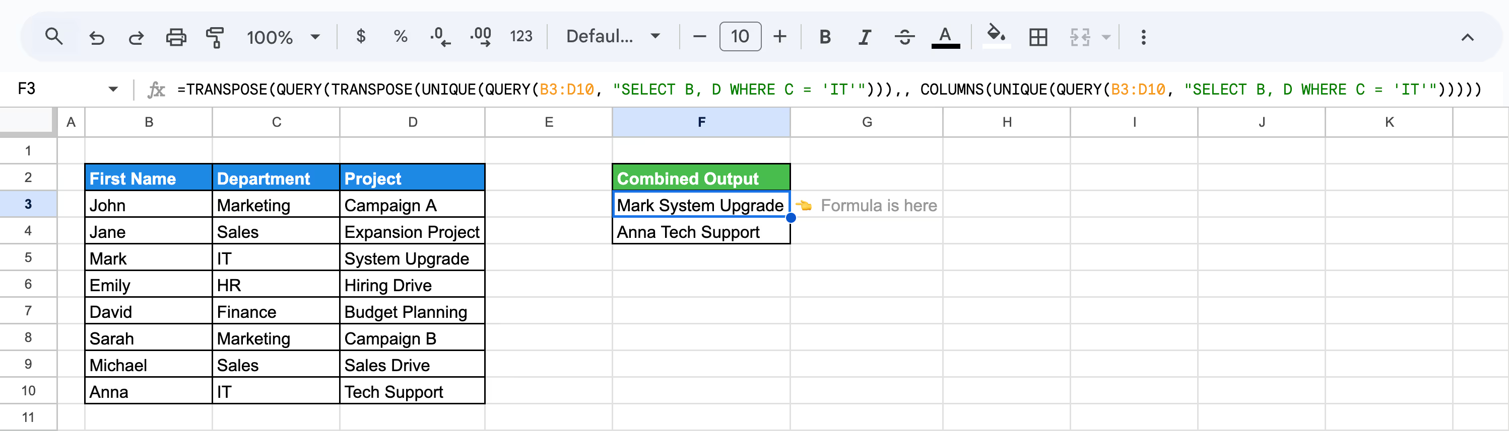
This formula efficiently combines filtered data and outputs it in a clean, summarized format, perfect for reporting or performance tracking in Google Sheets.
💡While combining text in Google Sheets using the & and CONCATENATE functions is powerful for straightforward text manipulations, incorporating QUERY with CONCATENATE can elevate your data handling. Dive into our guide on using QUERY with CONCATENATE in Google Sheets to unlock more advanced techniques for managing and analyzing your data seamlessly.


Using CONCATENATE with TODAY Function
The CONCATENATE function, combined with the TODAY function in Google Sheets, allows you to dynamically display the current date alongside text. This is ideal for creating reports, logs, or summaries that require real-time date updates. The TODAY function automatically refreshes the date each day.
The formula will be:
=CONCATENATE("Report generated on ", TEXT(TODAY(), "mm/dd/yyyy"))
Here’s the breakdown:
- "Report generated on ": Static text that will appear as the first part of the concatenated result.
- TODAY(): Returns the current date.
- TEXT(TODAY(), "mm/dd/yyyy"): Formats the current date (TODAY()) in the mm/dd/yyyy format.
- CONCATENATE: Combines the static text and the formatted date into one continuous string.
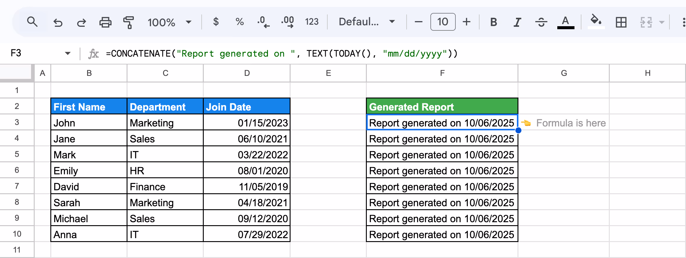
This approach simplifies the process of creating up-to-date reports or summaries, ensuring the inclusion of accurate, real-time dates.
Using CONCATENATE with COUNTA
The CONCATENATE function combined with the COUNTA function in Google Sheets helps you dynamically count non-empty cells and merge the result with descriptive text. This is particularly useful for summaries, such as counting team members, tasks, or entries.
Let's use the formula:
=CONCATENATE("Total employees in the list: ", COUNTA(B3:B10))
Here’s the breakdown:
- "Total employees in the list: ": Adds contextual text for clarity.
- COUNTA(B3:B10): Counts the number of non-empty cells in the specified range (First Name column).
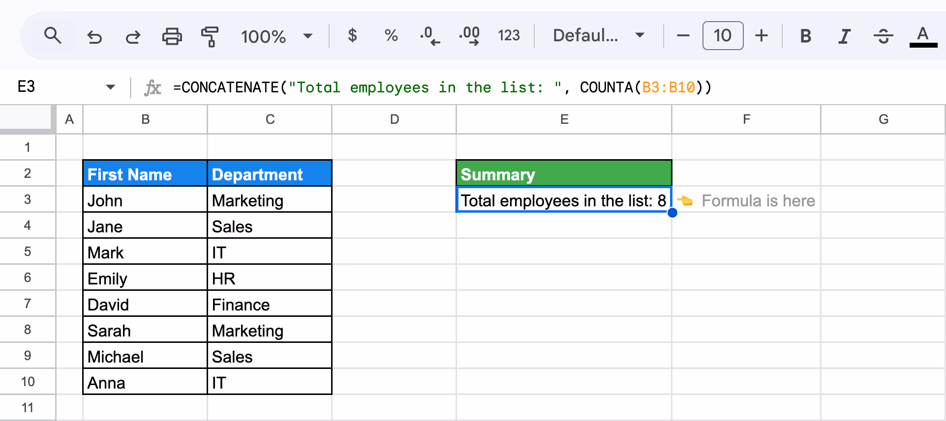
This method is ideal for creating quick summaries, like counting team members or active entries, and presenting the results in a clear, professional format.
💡Mastering text combination in Google Sheets sets a solid foundation for understanding more complex functions. To further enhance your data analysis skills, explore our detailed guide on the COUNT and COUNTA functions, which are crucial for quantifying data directly within your spreadsheets.

Using CONCATENATE with VLOOKUP and HLOOKUP
By combining VLOOKUP and HLOOKUP with the CONCATENATE function in Google Sheets, you can dynamically merge data from both vertical and horizontal searches into a meaningful summary. In this example, we create a sentence combining Mark's name (using VLOOKUP) and his corresponding Project.
The formula used is:
=CONCATENATE(VLOOKUP("Mark", B3:D10, 1, FALSE), " is assigned to ", HLOOKUP("System Upgrade", B5:D5, 1, FALSE))
Here’s the breakdown:
- VLOOKUP("Mark", B3:D10, 1, FALSE): Searches for "Mark" in the First Name column (B3:B10) and returns his name.
- HLOOKUP("System Upgrade", B5:D5, 1, FALSE): Searches for "System Upgrade" in the Project row (B5:D5) and retrieves the value.
- CONCATENATE: Combine these outputs with the text " is assigned to " for clarity.
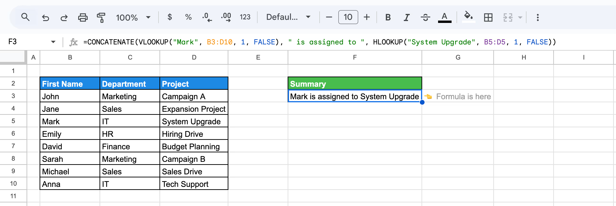
This method effectively demonstrates how VLOOKUP and HLOOKUP can work together to provide meaningful insights and organized outputs in Google Sheets.
Creating Dynamic Text with CONCATENATE and ROW
Using the CONCATENATE function with the ROW function in Google Sheets enables you to generate dynamic text entries, such as numbered lists or labels, based on row numbers. This is particularly useful for organizing data in reports, task lists, or sequential entries.
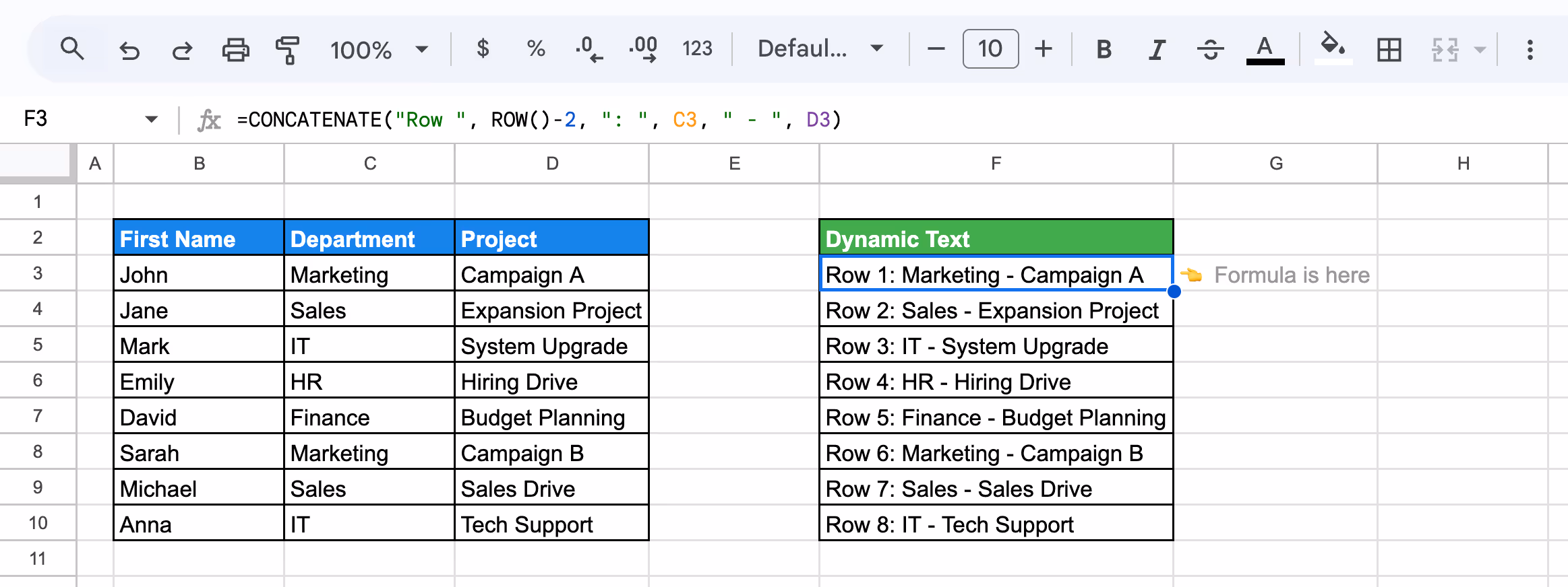
To create dynamic text entries combining the row number and values from columns, let’s use the next formula:
=CONCATENATE("Row ", ROW()-2, ": ", C3, " - ", D3)
Here’s the breakdown:
- ROW()-2: Returns the current row number minus an offset to adjust numbering.
- C3: Refers to the Department value.
- D3: Refers to the Project value.
- "Row " and " - ": Adds descriptive text and separators for better readability.
This approach simplifies the process of creating dynamic and professional text outputs while ensuring consistency across rows. It is perfect for managing lists, labels, and organized reports in Google Sheets.
Using CONCATENATE with CHAR for Line Breaks
The CONCATENATE function, combined with the CHAR function in Google Sheet,s enables you to insert line breaks within merged text. This is particularly useful for creating structured outputs like multi-line summaries, labels, or notes. The CHAR(10) value represents a line break in Google Sheets.
The formula used is:
=CONCATENATE(B3, CHAR(10), C3, CHAR(10), D3)
Here’s the breakdown:
- B3: Refers to the First Name.
- CHAR(10): Inserts a line break.
- C3: Refers to the Department.
- D3: Refers to the Project.
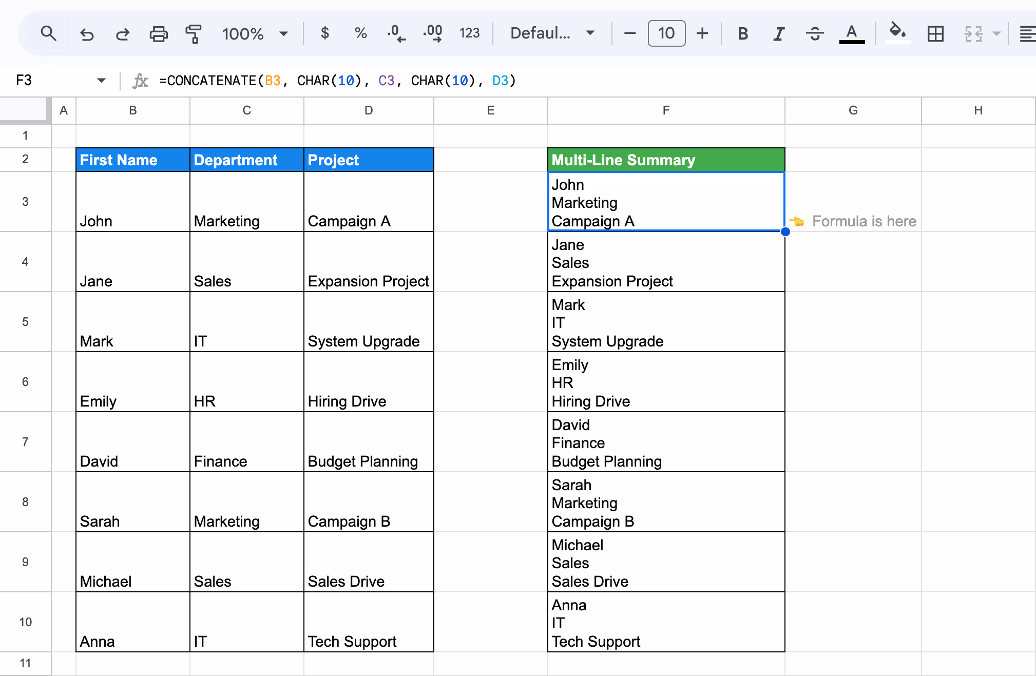
This method helps you present combined data in an organized and visually appealing multi-line format, improving clarity in reports and outputs.
Using CONCATENATE with SUM
Combining the CONCATENATE function with SUM in Google Sheets allows you to create dynamic text summaries with calculated results. This approach is ideal for generating summaries, such as total salaries, presented with descriptive text for clarity.
The formula will be:
=CONCATENATE("The total salary is $", SUM(C3:C10))
Here’s the breakdown:
- "The total salary is $": Static text that provides context.
- SUM(C3:C10): Calculates the total sum of the salary column.
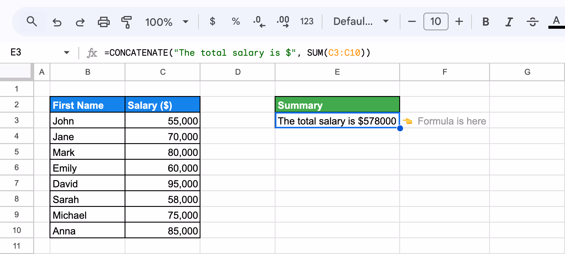
This method simplifies reporting by merging calculations, such as totals, with clear and dynamic text outputs, improving clarity and professionalism in your spreadsheets.
💡While the CONCATENATE function and the "&" operator help you merge text seamlessly in Google Sheets, understanding numerical data manipulation is just as crucial. Dive into our comprehensive guide on SUM functions to learn how to effectively aggregate numerical data in your spreadsheets.

Using ARRAYFORMULA with CONCATENATE
When using CONCATENATE with ARRAYFORMULA in Google Sheets, it attempts to combine entire ranges into a single output string rather than processing rows individually.
The formula used is:
=ARRAYFORMULA(CONCATENATE(B3:B10, " - ", C3:C10))
Here’s the breakdown:
- ARRAYFORMULA: Enables the formula to work on an entire range instead of a single cell.
- B3:B10: Refers to the range containing First Name values.
- " - ": Adds a separator between concatenated text.
- C3:C10: Refers to the range containing Department values.

In this case, instead of concatenating each row separately, all values in the First Name and Department columns are combined into one continuous text string, resulting in an unreadable output. The CONCATENATE function isn’t designed to handle array ranges row by row within ARRAYFORMULA. It processes the full range at once, producing a single, combined output.
To achieve row-by-row concatenation dynamically, you can use the & operator instead of CONCATENATE. The & operator works seamlessly with ARRAYFORMULA to produce clean, row-specific results.
You can discover more about how to fix this and improve your formula in the next example.
Dynamic Range Manipulation Using Ampersand with ARRAYFORMULA
The Ampersand operator combined with ARRAYFORMULA allows dynamic range manipulation in Google Sheets, enabling text to be added to the beginning, end, or in between cell values. This is particularly useful for applying transformations across multiple rows simultaneously without dragging formulas. Below are two variations that demonstrate this capability.
To add text dynamically at the start and end of a range of values in column B, use:
=ARRAYFORMULA("Employee: " & B3:B10 & " - Active")
Here’s the breakdown:
- "Employee: ": Static text added to the beginning of each value.
- B3:B10: The range containing the First Name column.
- " - Active": Static text added to the end of each value.

To include dynamic row numbers combined with cell values, use:
=ARRAYFORMULA("Row " & ROW(B3:B10) - 2 & ": " & B3:B10)
Here’s the breakdown:
- "Row ": Static text indicating the row label.
- ROW(B3:B10) - 2: Dynamically generates row numbers starting from 1.
- B3:B10: The range with values to concatenate.
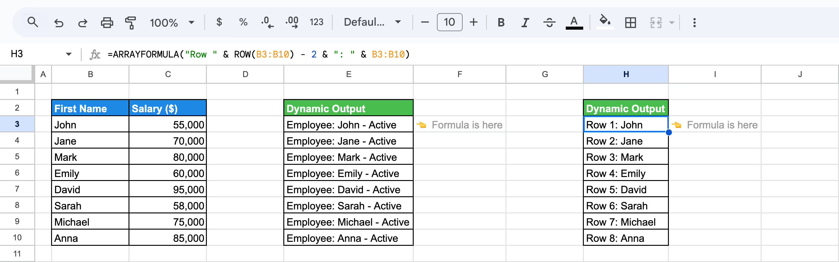
Using the Ampersand operator with ARRAYFORMULA simplifies dynamic range manipulation, enabling you to create clean and structured outputs for reports, labels, or task lists. This approach is far more effective than manually applying formulas row by row.
Dynamic Text Concatenation with Ampersand, IF, LEN, and ARRAYFORMULA
Combining the Ampersand operator with IF, LEN, and ARRAYFORMULA allows you to dynamically manipulate text based on specific conditions across multiple rows in Google Sheets. This approach is perfect for conditional text outputs, where values are modified based on their length, emptiness, or other criteria.
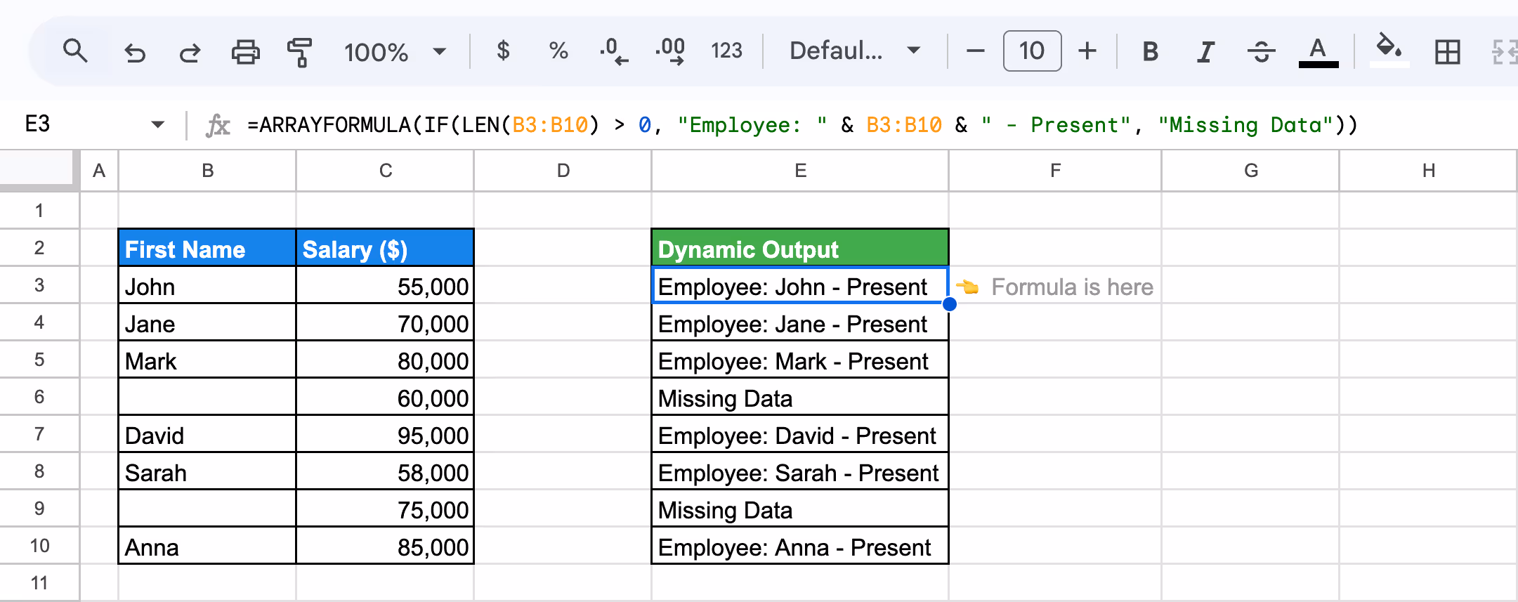
To add text only when a condition is met (e.g., the length of a value is greater than 0), use:
=ARRAYFORMULA(IF(LEN(B3:B10) > 0, "Employee: " & B3:B10 & " - Present", "Missing Data"))
Here’s the breakdown:
- LEN(B3:B10) > 0: Checks if the length of each cell in the range B3:B10 is greater than 0 (i.e., not empty).
- "Employee: " & B3:B10 & " - Present": Adds text to the beginning and end of each cell where the condition is met.
- "Missing Data": Returns this text if the condition is false (cell is empty).
- ARRAYFORMULA: Processes the entire range dynamically.
This method showcases the power of Ampersand, IF, LEN, and ARRAYFORMULA to automate conditional text concatenation, making it an ideal solution for data validation, reporting, or labeling in Google Sheets.
Troubleshooting Common Issues with CONCATENATE
Troubleshooting common issues with the CONCATENATE function in Google Sheets involves identifying and resolving errors that arise from improper syntax, invalid references, or incompatible data types. By understanding the root causes of these issues, you can streamline your workflow and ensure accurate results when combining text strings.
#VALUE! Error
⚠️ Error: The #VALUE! error occurs in the CONCATENATE function when it encounters incompatible data types, such as attempting to combine a cell containing a formula error or invalid characters. This error can also appear if the function references blank or non-text cells unexpectedly.
✅ Solution: Verify that all referenced cells contain valid text, numbers, or data that can be converted into strings. If needed, use functions like TEXT() to standardize data formatting or ISBLANK() to handle empty cells before concatenation.
#REF! Error
⚠️ Error: The #REF! error occurs in the CONCATENATE function when it references a cell that has been deleted or if the formula contains an invalid cell reference. This error can also appear when moving or modifying sheets that disrupt linked references.
✅ Solution: Check your formula for broken or missing references and ensure all referenced cells exist. If a referenced cell was accidentally deleted, restore it or update the formula to point to the correct range. Use absolute references where necessary to prevent errors caused by moving data.
#N/A Error
⚠️ Error: The #N/A error occurs in the CONCATENATE function when it references a cell containing the #N/A value, often caused by lookup errors or missing data. This error indicates that the function cannot process the unavailable value as part of the concatenation.
✅ Solution: Identify and resolve the source of the #N/A value in the referenced cells by verifying the lookup or formula producing the error. Use functions like IFERROR() or IFNA() to handle missing data gracefully, replacing #N/A values with blank text ("") or default placeholders before concatenation.
#NAME? Error
⚠️ Error: The #NAME? error occurs in the CONCATENATE function when there is a typo in the function name, missing quotation marks around text values, or unrecognized names in the formula. This error indicates that Google Sheets cannot interpret the formula as written.
✅ Solution: Check the formula for typos in the function name or syntax errors, such as missing quotation marks around text strings. Ensure all function names and parameters are correctly spelled and formatted. If referencing a named range, verify its existence and correct spelling.
#NUM! Error
⚠️ Error: The #NUM! error occurs in the CONCATENATE function when it encounters an invalid numeric operation, such as attempting to concatenate overly large numbers or improperly formatted numeric values. This error can also arise from exceeding formula limitations.
✅ Solution: Verify that all numeric values are properly formatted and within acceptable ranges. If necessary, use the TEXT() function to convert numbers into text before concatenation. Additionally, ensure the formula does not exceed Google Sheets' limits on cell references or input size.
Best Practices for Using CONCATENATE and Ampersand Functions
When combining text in Google Sheets, prioritize clarity, flexibility, and ease of use. Choose methods that suit your specific needs, whether it’s creating simple formulas or managing more complex data arrangements. Aim to keep your results organized and adaptable, ensuring they remain easy to read, adjust, and apply across various scenarios. By focusing on simplicity and scalability, you can streamline your work and enhance the effectiveness of your spreadsheets.
Use Ampersand as a Faster and Simpler Alternative to CONCATENATE
The ampersand (&) operator provides a streamlined and efficient alternative to the CONCATENATE function for combining text in Google Sheets. Its simplicity makes it an intuitive choice for many users, as it eliminates the need to type out longer function names. Instead, the ampersand allows you to quickly join text or values within a formula with minimal effort.
This approach is not only faster, but also easier to remember, especially when working on repetitive or complex tasks. By using the ampersand, you can save time and maintain clarity in your spreadsheet formulas, making it a preferred option for those seeking a more straightforward method for text concatenation.
Experimenting with Delimiters
Experimenting with delimiters is an essential step when combining text in Google Sheets. Delimiters, such as spaces, commas, or other symbols, help separate the joined values, making the results clearer and more readable. Maintaining consistency in the use of delimiters throughout your spreadsheet is crucial to avoid confusion and ensure the data remains organized.
Thoughtfully choosing and testing different delimiters can enhance the presentation and usability of your concatenated text, especially when dealing with complex datasets or creating reports.
Handling Empty Cells in Joined Data
Handling empty cells is an important consideration when joining data in Google Sheets. By default, some functions, like JOIN, skip empty cells, but this behavior may not always align with your desired outcome. To ensure consistent results, you can use functions such as IF or IFERROR to manage empty cells before combining them.
Gracefully handling empty cells prevents unintended gaps or formatting issues in your data. Being proactive about addressing empty cells ensures your concatenated text remains clear, accurate, and aligned with the overall structure of your spreadsheet.
Use Cell References Instead of Hardcoded Text
Using cell references instead of hardcoded text is a best practice when combining data in Google Sheets. Cell references make your formulas more dynamic and easier to update, as any changes to the referenced cells are automatically reflected in the results.
This approach not only saves time but also reduces the risk of errors when editing or expanding your data. By avoiding hardcoded text, you ensure that your spreadsheet remains flexible, scalable, and easier to manage in the long run.
Use Text Formatting
Incorporating text formatting into your concatenation formulas can significantly enhance the presentation of your data in Google Sheets. By combining the CONCATENATE function with tools like TEXT, you can control how numbers, dates, or other values appear in the final output.
Formatting options allow you to align the combined data with your desired style, improving readability and ensuring consistency. Thoughtful use of text formatting can make your spreadsheets more polished and professional, especially when preparing data for reports or sharing with others.
Make Sense of Your Data with OWOX: Reports, Charts, and Pivot Tables
While the & operator and the CONCATENATE function simplify text combination, managing complex datasets requires more robust tools. The OWOX: Reports, Charts & Pivots Extension streamlines your workflow by automating reporting, creating dynamic charts, and handling data integration effortlessly.
Save time on manual tasks and focus on deriving actionable insights. Install the OWOX Reports Extension for Google Sheets today to transform how you manage and analyze your data!
Frequently asked questions


Finally, a tool that doesn't ask business users to learn a new dashboarding UI. Our marketing team already knows Sheets. OWOX just delivers the right data.
Joinable data marts concept was the thing that sold us. We can now use the semantic layer without building one.
Self-hosted the OSS version on Digital Ocean. Zero vendor lock-in. Contributed a Shopify connector back in week two.