How to Search in Google Sheets: Tips and Shortcuts

Finding the right data in a big Google Sheet can be tricky, especially when you have lots of rows or different tabs. Google Sheets has some easy tools that help you search for names, numbers, or words, saving you time and effort. These features make it easier to spot what you’re looking for without having to scroll too much. 

Here’s how to search in Google Sheets more effectively, with tips and shortcuts to save time. In this guide, you’ll learn simple ways to search in Google Sheets using shortcuts, built-in tools, and formulas. Whether you’re just getting started or using spreadsheets every day, these tips will help you find things faster and work more smoothly.

Why Searching in Google Sheets Is Helpful

When you're working with a lot of data in Google Sheets, finding something specific can take a lot of time. The search features help you find exactly what you need without going through every row and column.

• Saves time: Quickly find the data you need without scrolling through hundreds of rows.
• Reduces errors: Spot mistakes or missing entries faster by jumping straight to the right cell.
• Improves focus: Helps you zero in on the most important information without distractions.
• Makes updates easier: Easily find and change values like names or numbers in just a few clicks.
• Supports better decisions: Having the right data in front of you leads to faster and smarter choices.

How to Search in Google Sheets: Tips and Shortcuts with This Ready-to-use Template!

This downloadable file contains all the examples from the article, allowing you to practice and implement How to Search in Google Sheets: Tips and Shortcuts in your own projects. Download, explore, and start mastering text wrapping techniques in Google Sheets with ease!

Download your FREE template today!

Basic Search Techniques in Google Sheets 

Basic search methods in Google Sheets help you quickly find specific data without scrolling through large tables. Whether you're looking for a name, product, or number, these simple tools make it easier to locate information and work more efficiently.

Using Ctrl + F (Windows) or Command + F (Mac)

To quickly find something in your sheet, use Ctrl + F for Windows and Command + F for Mac systems. A search bar appears at the top right.

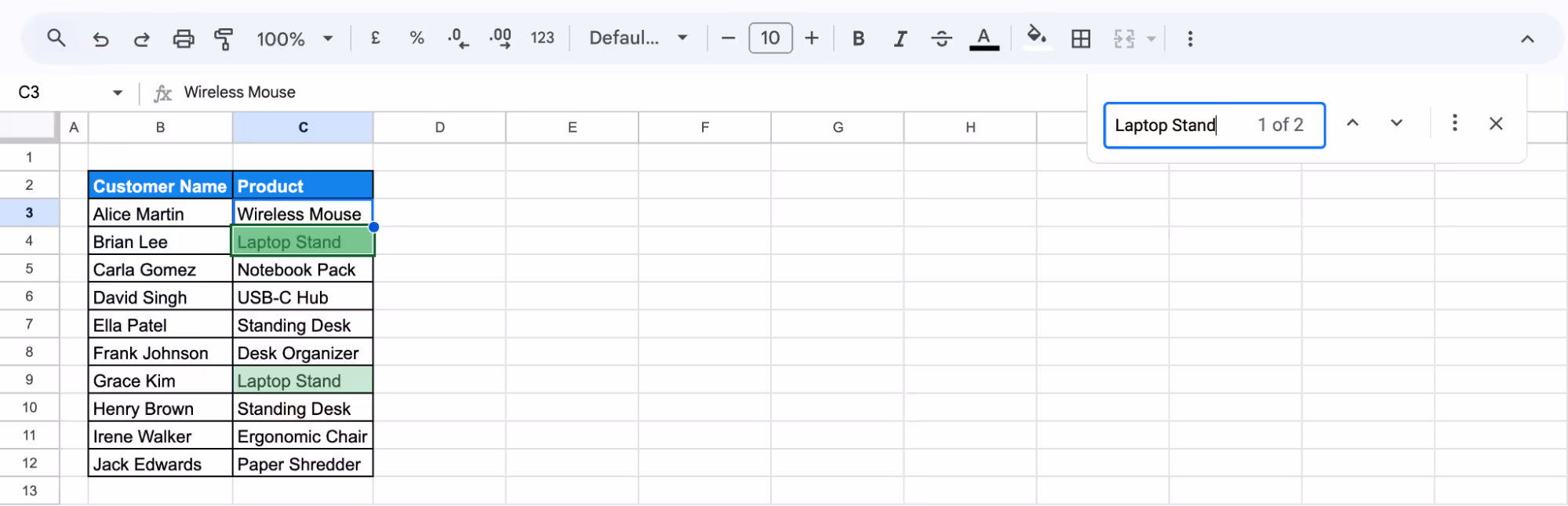
Example:

Suppose you have a dataset and want to find who purchased a Laptop Stand. Press Ctrl + F or Command + F and type “Laptop Stand” into the search bar, and Google Sheets will highlight the matching cells instantly.

Using the Find and Replace Tool 

The Find and Replace tool in Google Sheets helps you locate specific text or values and quickly update them across your sheet. It’s useful when you need to make changes in multiple places at once. Here are two ways to access it:

1. Using the keyboard shortcut

To open the Find and Replace tool quickly, press Ctrl + H on Windows or Command + Shift + H on Mac. This shortcut brings up a dialog box where you can search for specific words or values and replace them.

Example:

Suppose you want to find all products named Standing Desk. Type Standing Desk in the Find field, and you can choose to search in just this sheet, all sheets, or a specific range.

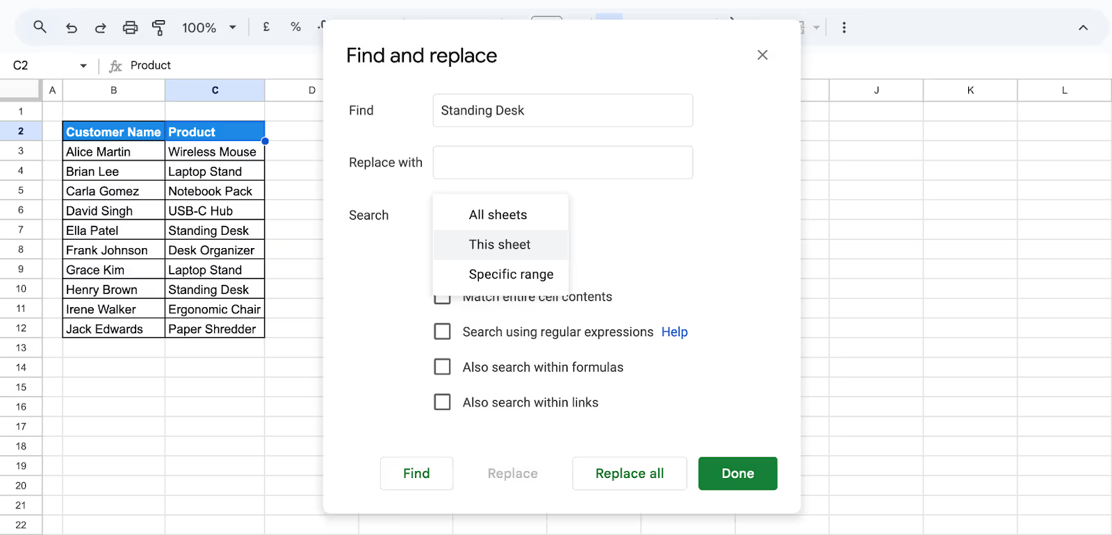
Now click Find to begin the search, and it will highlight each matching result one at a time.

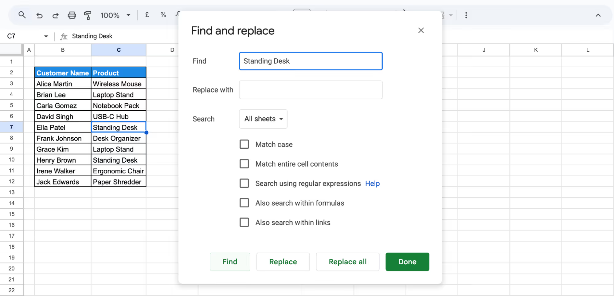
2. Using the find and replace tool

To access the Find and Replace tool in Google Sheets, go to the top menu and click Edit > Find and Replace.

When you click on the Find and Replace option, a dialog box will appear. 

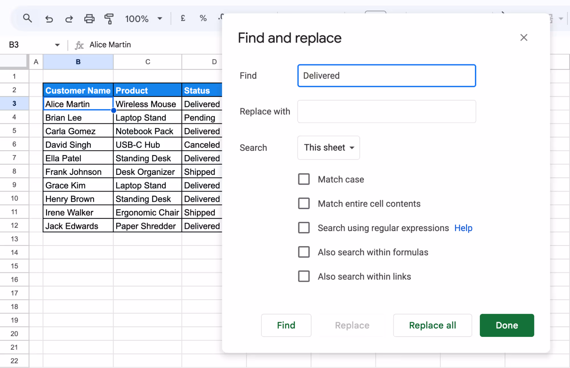
Example:

If you want to check the delivery status of products, type Delivered in the Find field, select This sheet as the search range and click Find. It will highlight each matching result one at a time.

💡 Want to make your spreadsheets more dynamic and easier to manage? Check out OWOX’s guide to the new Tables feature in Google Sheets to learn how to organize, filter, and analyze your data faster with built-in structure and flexibility.

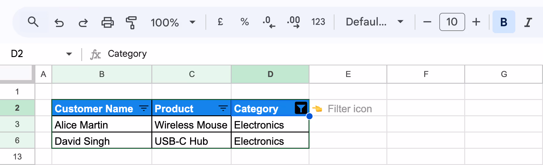
Searching with Filters for Quick Data Lookup

Filters help you find what you need by hiding data that doesn’t match your search. To use them, select the row with your headers, go to Data > Create a filter.

Click the filter icon on the column you want to search.

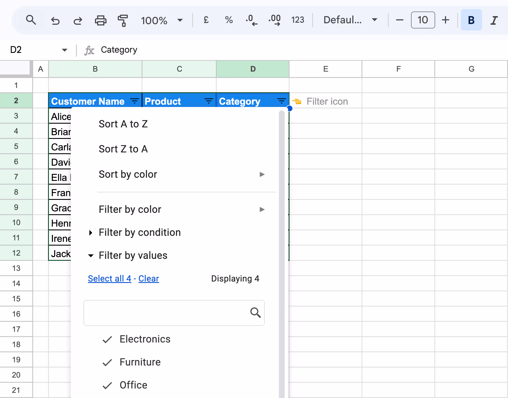
Example:

If you want to see only the customers who purchased electronic products, clear all selections and select Electronics from the list.

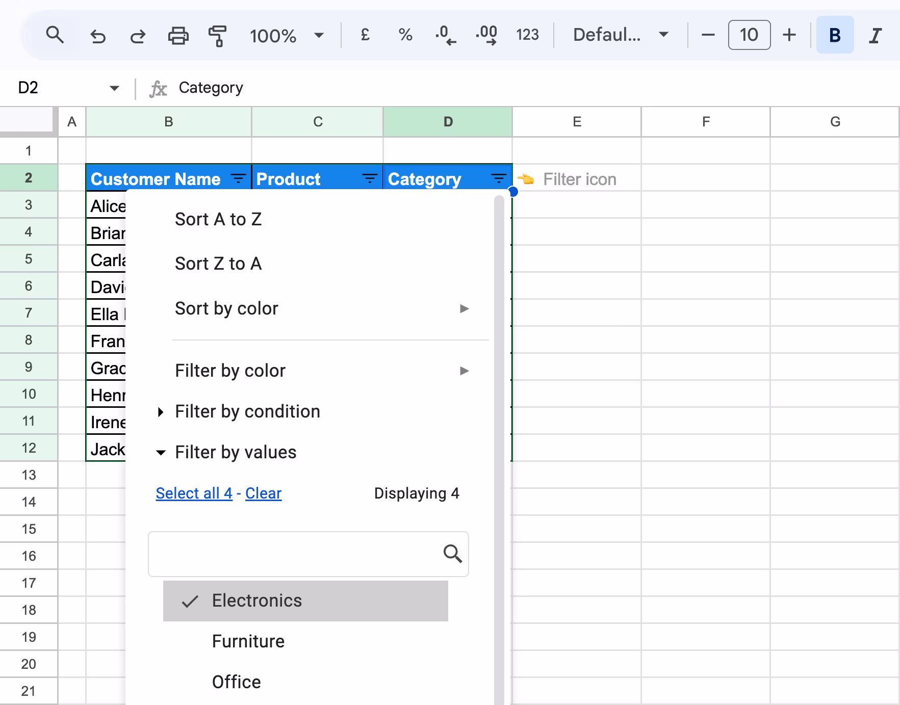
Press OK to apply the filter and view only the matching rows.

Using Conditional Formatting for Search

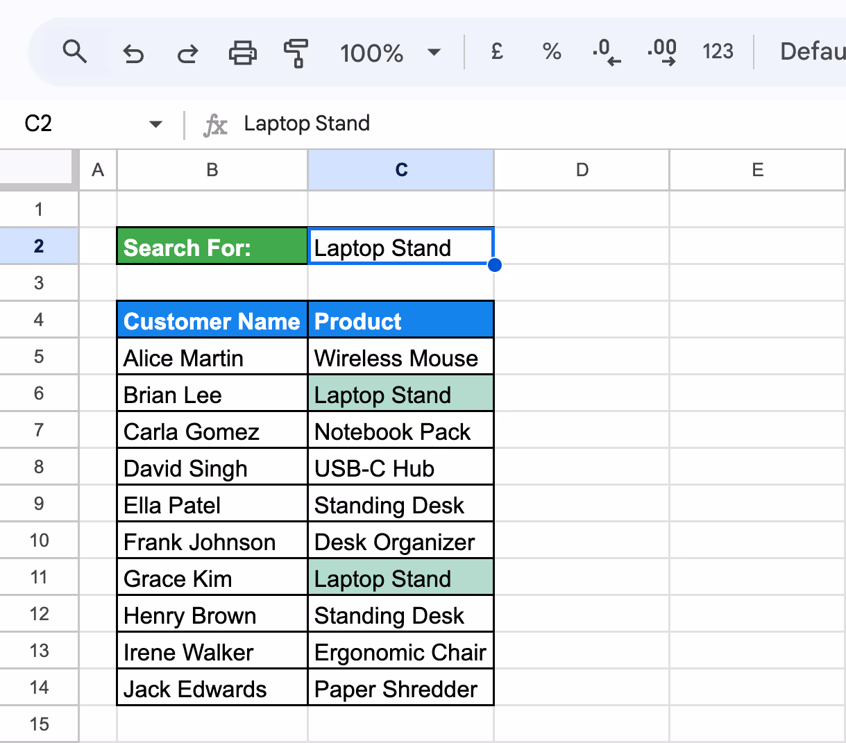
Conditional formatting helps highlight matching search results in your sheet. First, we will move the entire spreadsheet three rows down to create space at the top for adding the custom search bar and select the range you want to search in. Then go to Format > Conditional Formatting from the top menu.

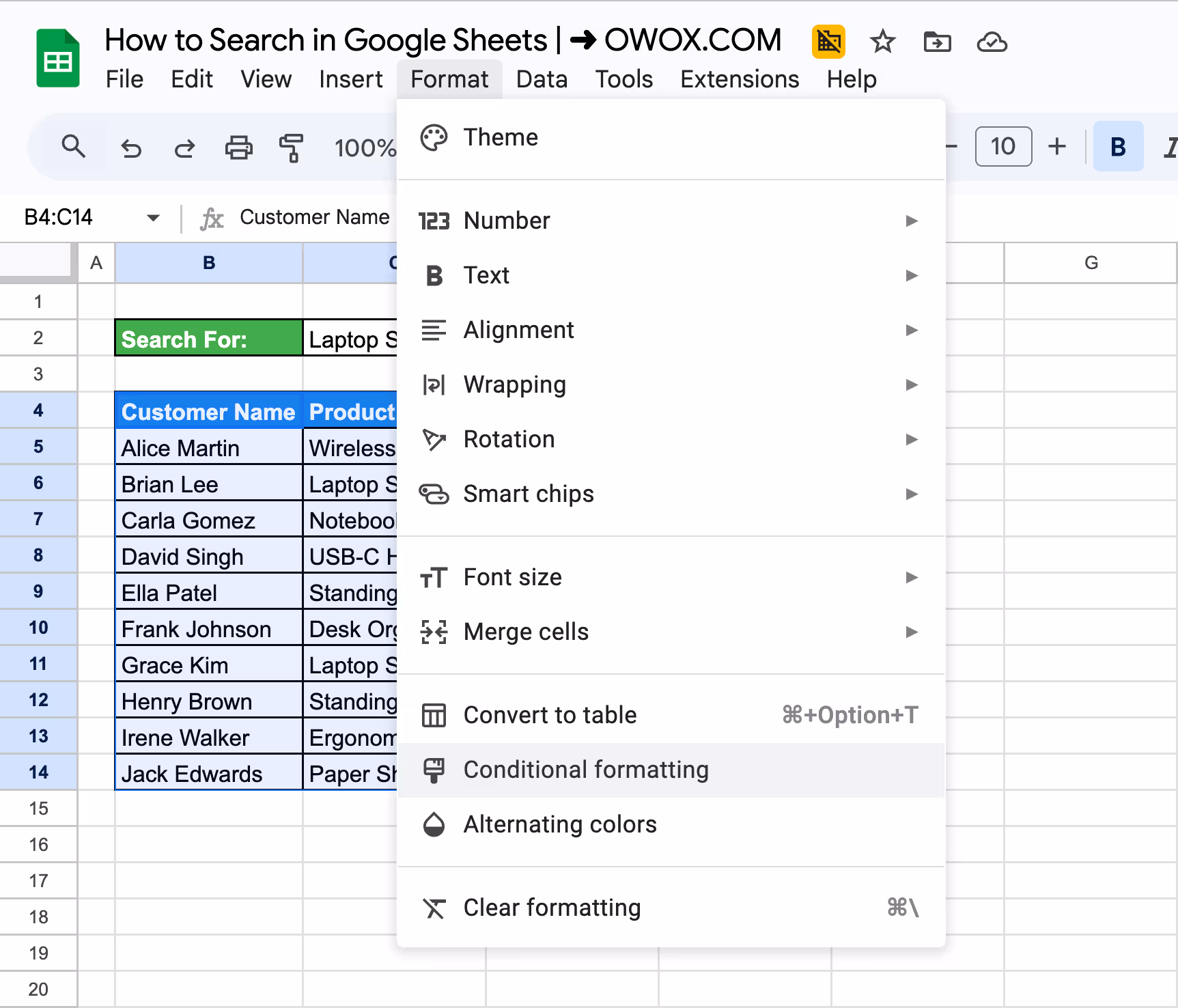
The Conditional Formatting bar will appear on the right-hand side. In the Format cells if section, choose Custom formula is, and enter the below formula.

=ISNUMBER(FIND($C$2,B5))

Here's what each parameter means:

• $C$2 refers to the value you're searching for.
• B5 refers to the cell you're searching in - the formula checks if the value from $C$2 exists within cell B5.

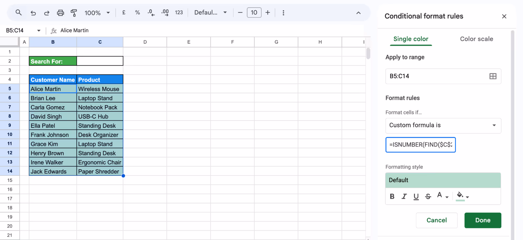
Example:

Suppose you want to search for “Laptop Stand,” simply type it into the search bar (cell C2) and press Enter. The matching cells will be highlighted automatically.

Advanced Search Techniques to Use in Google Sheets

Advanced search techniques in Google Sheets help you go beyond simple lookups. With these methods, you can search across multiple sheets, apply custom logic, and automate your searches for faster, more accurate results in larger or more complex datasets.

Enhancing Google Sheets Search with Add-ons

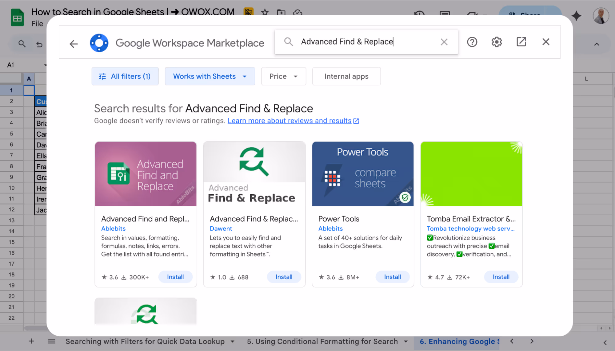
Add-ons can improve search in Google Sheets, especially when built-in tools aren’t enough. To get one, go to the Extensions > Add-ons > Get add-ons menu.

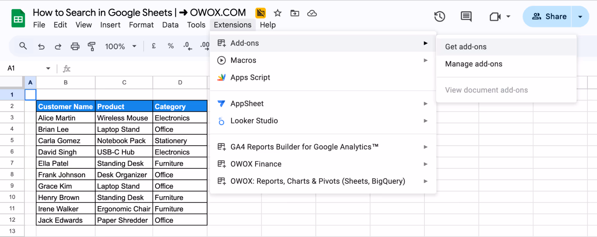
Search for tools like Power Tools or Advanced Find & Replace that are designed to make searching and managing data easier.

After installing, you’ll find them under the Add-ons menu for easy access and extra features.

Automating Advanced Searches with Google Apps Script

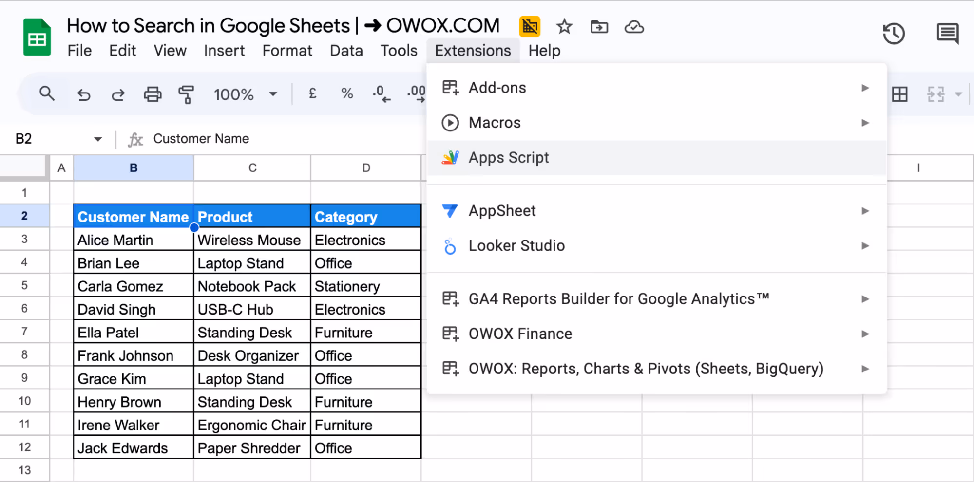
Google Apps Script lets you create custom search functions when you need more control than standard tools allow. To get started, go to Extensions > Apps Script in your Google Sheet.

Example:

You have a dataset listing customer purchases, including the Customer Name, Product, and Category. You want to quickly find all entries where a specific keyword appears in the Product column - for example, finding all items that include “Mouse”.

In the script editor, you can write a custom search using JavaScript. 

1function searchProductName() {
2  const sheet = SpreadsheetApp.getActiveSpreadsheet().getActiveSheet();
3  const searchValue = sheet.getRange("F3").getValue(); // ✅ Use a cell outside the data table
4  const headerRow = 2;
5  const startRow = headerRow + 1; // Start from row 3
6  const productCol = 3; // Column C (Product)
7
8  const lastRow = sheet.getLastRow();
9  const lastColumn = sheet.getLastColumn();
10  const dataRange = sheet.getRange(startRow, 2, lastRow - headerRow, lastColumn - 1); // Start from column B
11  const data = dataRange.getValues();
12
13  // Clear formatting only in the data range (not header)
14  dataRange.setBackground(null);
15
16  for (let i = 0; i < data.length; i++) {
17    const productName = data[i][productCol - 2]; // Adjusted for range starting at column B
18    if (typeof productName === 'string' && productName.toLowerCase().includes(searchValue.toLowerCase())) {
19      const rowRange = sheet.getRange(startRow + i, 2, 1, lastColumn - 1);
20      rowRange.setBackground('#c6efce'); // Light green for match
21    }
22  }
23}

‍

Instead of manually scanning the list or using filters, this would automate the process- when a keyword is entered in cell C2, the script searches the Product column for that keyword (case-insensitive) and highlights any matching rows in green. This makes it easier to visually identify relevant entries without using filters or formulas.

‍

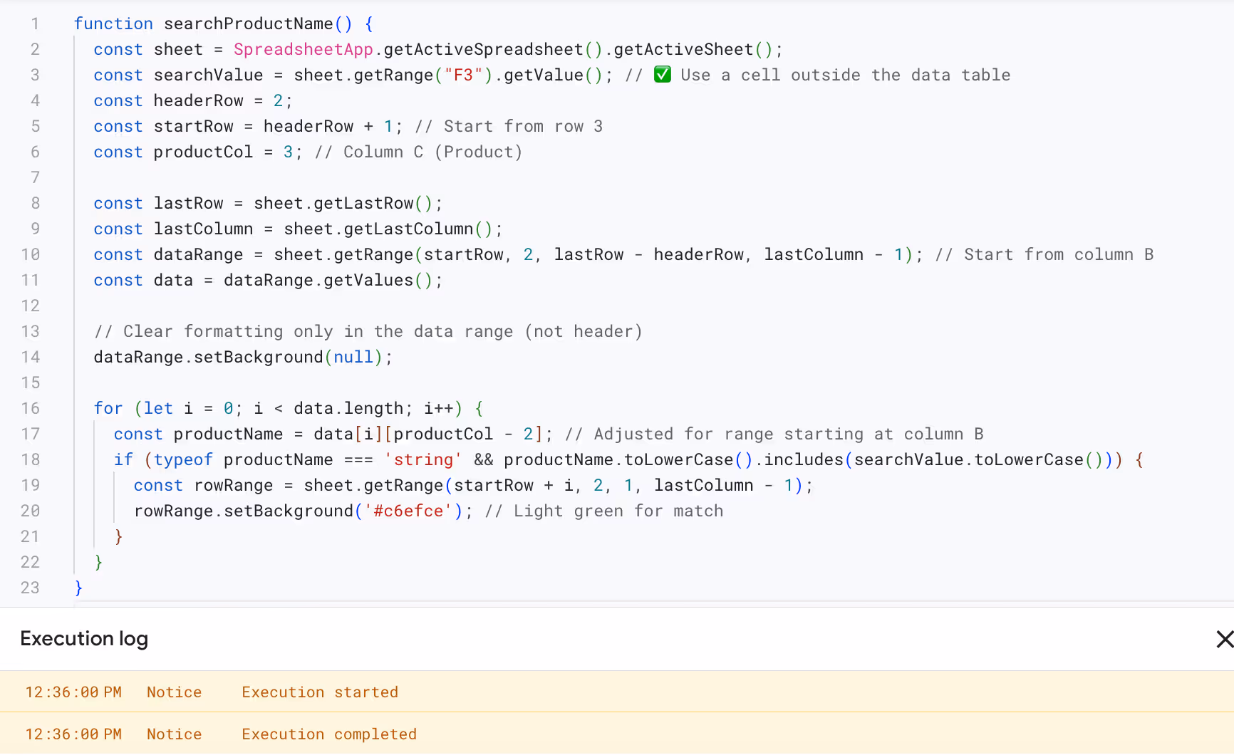
Though this method requires basic coding knowledge, it’s powerful for automating advanced searches or connecting with other Google services.

💡 Looking to present your data clearly and effectively? Explore OWOX’s guide to creating Bar Graphs in Google Sheets, discover how to build visual comparisons, and highlight key insights in seconds.‍

Searching Data in Google Sheets Using Functions

Google Sheets offers several built-in functions that make it easy to search through your data. These functions help you find values, filter rows, or return matching results based on specific criteria, making data analysis faster and more accurate.

MATCH Function

The MATCH function helps you find the position of a value in a column or row. It’s useful when you need to know where a specific item appears in your data.

Syntax:

=MATCH(search_key, range, [search_type])

Here's what each parameter means:

• search_key: The value you’re looking for.
• range: The range of cells where you want to search.
• search_type: Optional. Use 0 for an exact match.

Example:

Suppose you want to find the position of "Ella Patel" in the Customer Name column (B2:B11). You can use the following formula:

=MATCH("Ella Patel", B2:B12, 0)

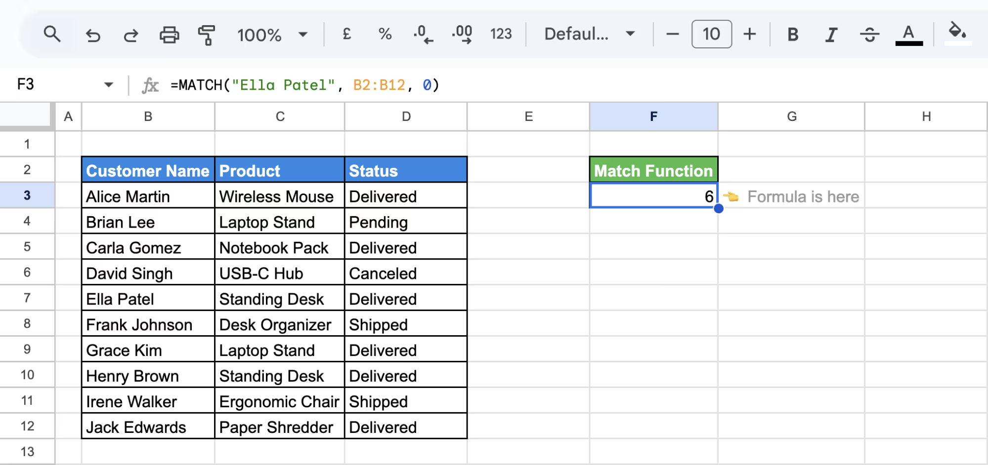
This will return 6, meaning Ella Patel is the sixth item in the selected range.

VLOOKUP Function

The VLOOKUP function helps you find a value in the first column of a range and return related data from another column in the same row. 

Syntax:

=VLOOKUP(search_key, range, index, [is_sorted])

Here's what each parameter means:

• search_key: The value you want to look up.
• range: The table range that includes the data you want.
• index: The column number (starting from 1) in the range to return the value from.
• is_sorted: Optional. Use FALSE for exact matches.

Example:

Suppose you want to find the price of USB-C Hub from the dataset (C2:E12). You can use the formula:

=VLOOKUP("USB-C Hub", C2:E12, 3, FALSE)

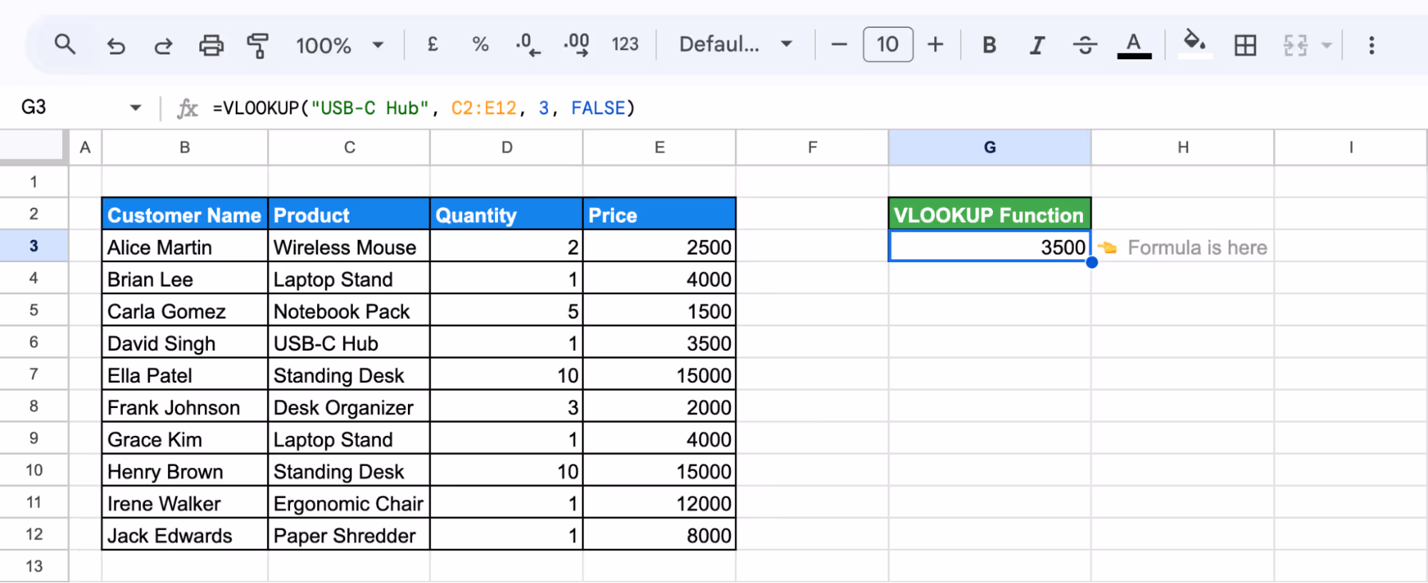
This will return 3500, which is the price listed in the third column (Price) of the matching row for USB-C Hub.

FILTER Function

The FILTER function helps you pull only the rows that meet certain conditions. It’s useful when you want to view a specific part of your data without manually sorting or hiding other entries.

Syntax:

=FILTER(range, condition1, [condition2, ...])

Here's what each parameter means:

• range: The range of data you want to return.
• condition1: The main rule that decides which rows to show.
• condition2, ...: Extra rules to narrow down the result (optional).

Example:

Suppose you want to display all orders where the price is greater than 10,000. You can use the following formula:

=FILTER(B2:E11, E2:E11 > 10000)

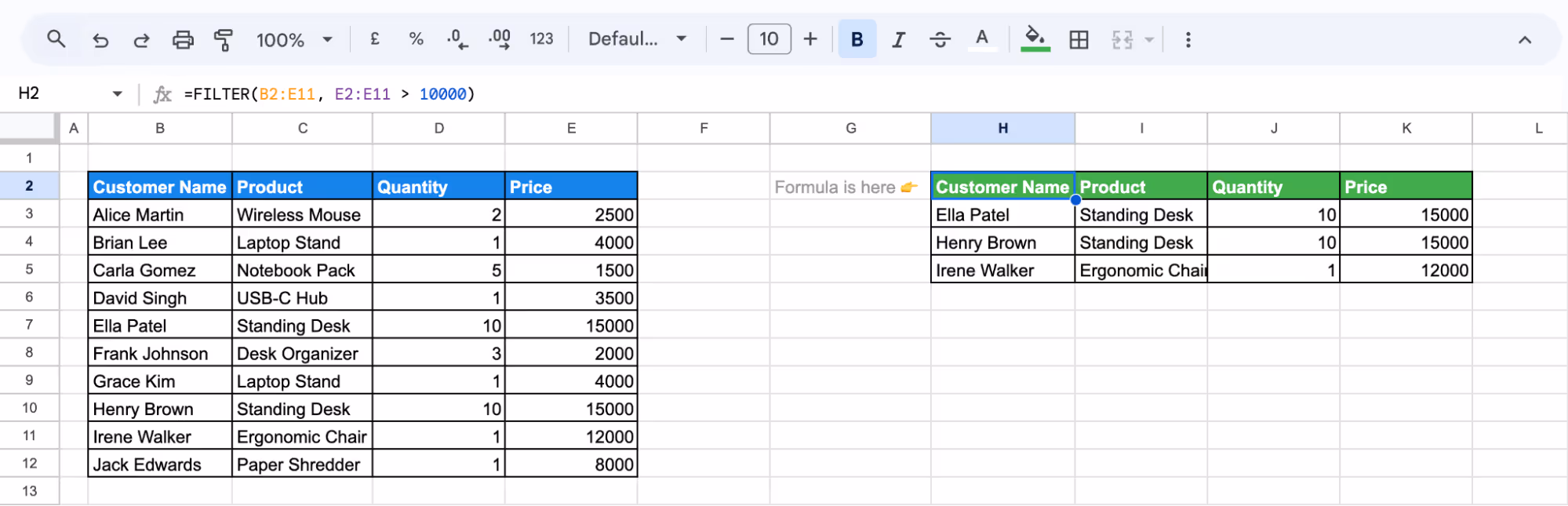
This will return only the rows where the price exceeds 10,000, helping you focus on high-ticket items in your sales data.

QUERY Function

The QUERY function lets you filter and sort data using SQL-like statements. It’s powerful for advanced searches, especially when you want specific rows based on text, numbers, or categories all in a single formula.

Syntax:

=QUERY(data, query, [headers])

Here's what each parameter means:

• data: The full range of cells you want to run the query on.
• query: A text string written in query language (like SQL).
• headers: Optional. The number of header rows (use 1 if your first row has column titles).

Example:

Suppose you want to list all customers who purchased items from the Furniture category. You can use the formula:

=QUERY(B2:D12, "SELECT B, C WHERE D = 'Furniture'", 1)

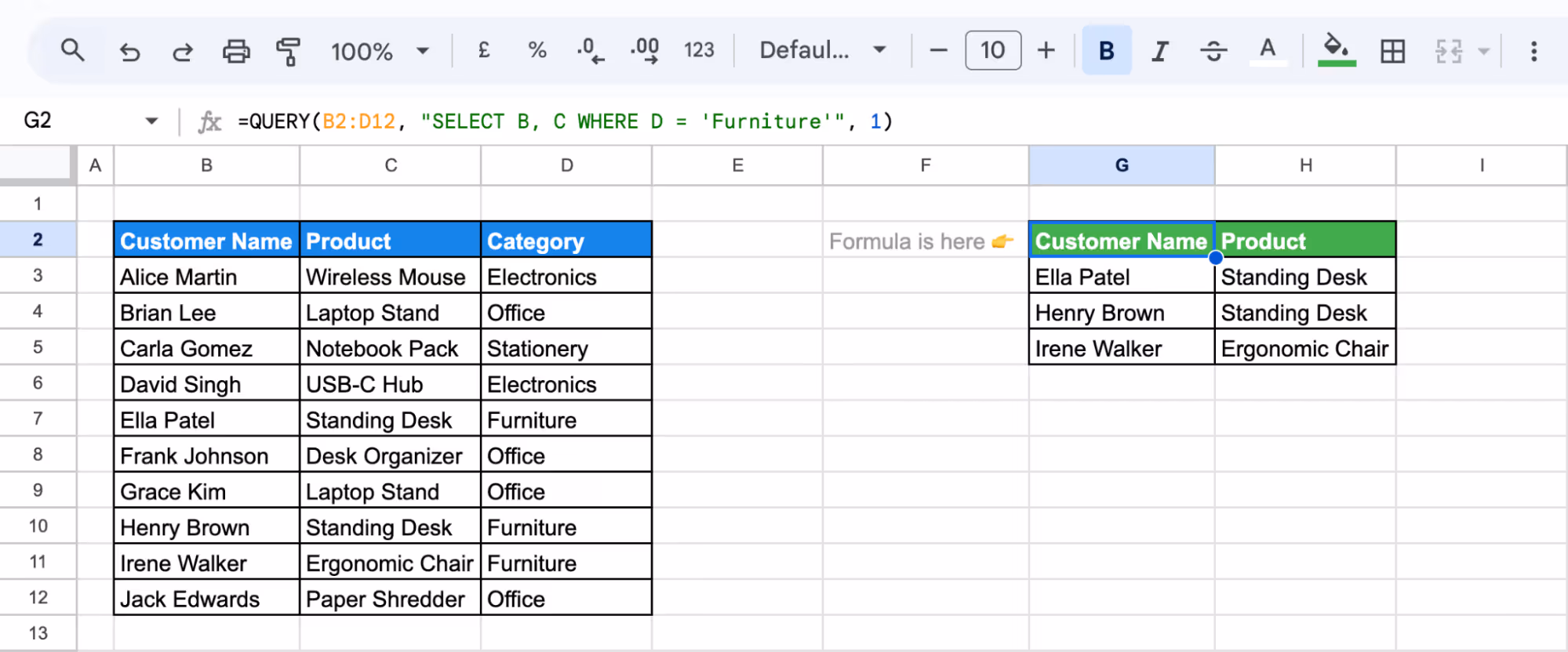
This will return only the Customer Name and Product columns where the Category is Furniture.

SEARCH Function

The SEARCH function helps locate the position of a word or phrase inside a cell. It's especially useful for checking if a review includes specific keywords without scanning each row manually.

Syntax:

=SEARCH(search_for, search_cell, [start_at])

Here's what each parameter means:

• search_for: The word or phrase you want to find.
• search_cell: The cell that contains the text you want to search in.
• start_at: Optional. Where to begin the search (defaults to character 1 if not used).

Example:

Suppose you want to find out if the word "comfortable" appears in the review written in cell D8, which says, "Very comfortable angle for working on a desk." Use the following formula:

=SEARCH("comfortable", D9)

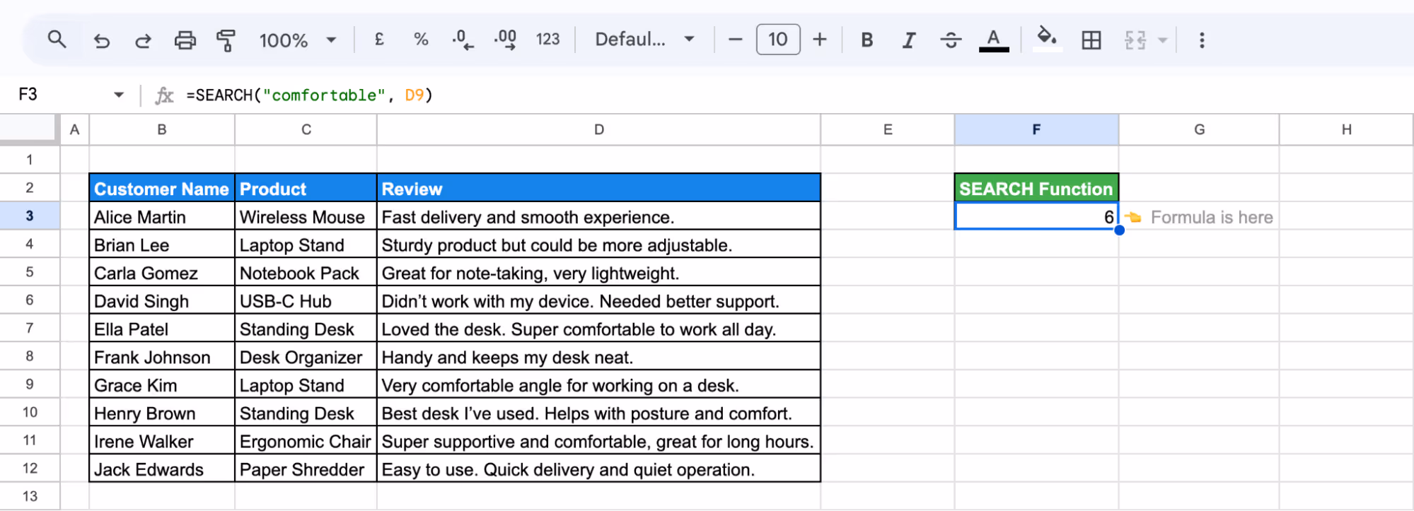
This will return 6, meaning the word comfortable starts at the 6th character of the text in that cell.

REGEX Functions

The REGEXMATCH function checks if a cell contains a specific pattern or word using regular expressions. It returns TRUE if there's a match and FALSE if not. This is useful when searching for multiple values or similar text variations in a single column.

Syntax:

=REGEXMATCH(text, regular_expression)

Here's what each parameter means:

• text: The cell you want to check.
• regular_expression: The pattern or keyword(s) you're trying to match.

Example:

Suppose you want to check the status in cells which contain either "Delivered" or "Shipped". You can use the following formula:

=REGEXMATCH(D3, "Delivered|Shipped")

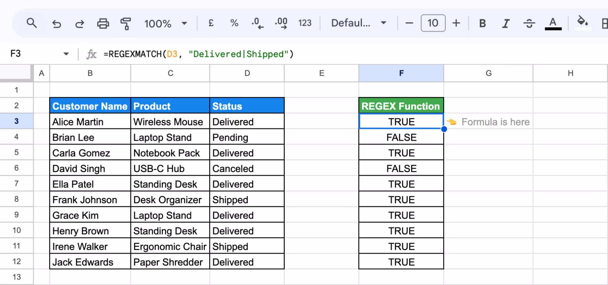
This formula quickly shows which rows have a status of "Delivered" or "Shipped" by returning TRUE.

IMPORTRANGE Function

The IMPORTRANGE function lets you pull data from another sheet or even a different Google Sheets file. It’s especially helpful when your data is spread across multiple sources and you want to search or analyze it in one place.

Syntax:

=IMPORTRANGE(spreadsheet_url, range_string)

Here's what each parameter means:

• spreadsheet_url: The full URL of the source spreadsheet (in quotes).
• range_string: The specific range you want to import, including the sheet name (also in quotes).

Example:

Suppose you want to pull data from another file and search for a specific order. You can combine IMPORTRANGE with QUERY like this:

=QUERY(IMPORTRANGE("hhttps://docs.google.com/spreadsheets/d/1A-J2kdZfgGgpJL61XOyTS_3Sa8tzqHk1BD_XFtrDL9o/edit?gid=1455503713#gid=1455503713", "Sheet1!B2:D"), "SELECT * WHERE Col1 = 'Alice Martin'")

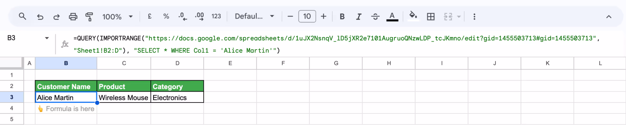
This formula will fetch data from Sheet1 in another spreadsheet and return all rows where Column 1 contains Alice Martin.

FIND Function

The FIND function returns the position of a specific word or character inside a cell’s text. Unlike SEARCH, it's case-sensitive, so it only works when the case matches exactly. 

Syntax:

=FIND(search_for, search_text, [start_at])

Here's what each parameter means:

• search_for: The exact word or letter you're trying to find.
• search_text: The cell where you want to look for it.
• start_at: Optional. Tells the function where to begin the search.

Example:

If you want to search the word "comfortable" in the review from cell D9, and the search term is typed in cell F3, use the formula:

=FIND(F3, D9)

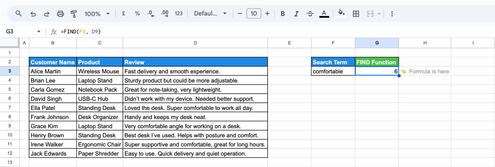
This returns 6, meaning the word comfortable starts at the 6th character in the text. Since the case of both the search term and the review match exactly, the formula works successfully.

How to Build a Search Box in Google Sheets 

Creating a search box in Google Sheets makes it easy to filter and find specific data without scrolling through rows manually. With a few simple steps, you can set up a dynamic search bar that updates results based on user input.

Creating a Dynamic Search Box with QUERY and Data Validation

Create a dynamic search box in Google Sheets using QUERY and Data Validation to let users choose how to search and instantly see filtered results based on their input.

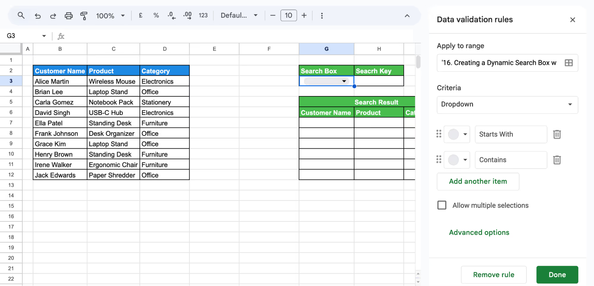
First, assign cells for the search type, search term, and result display. Then select G3, go to the Data menu, and click Data validation.

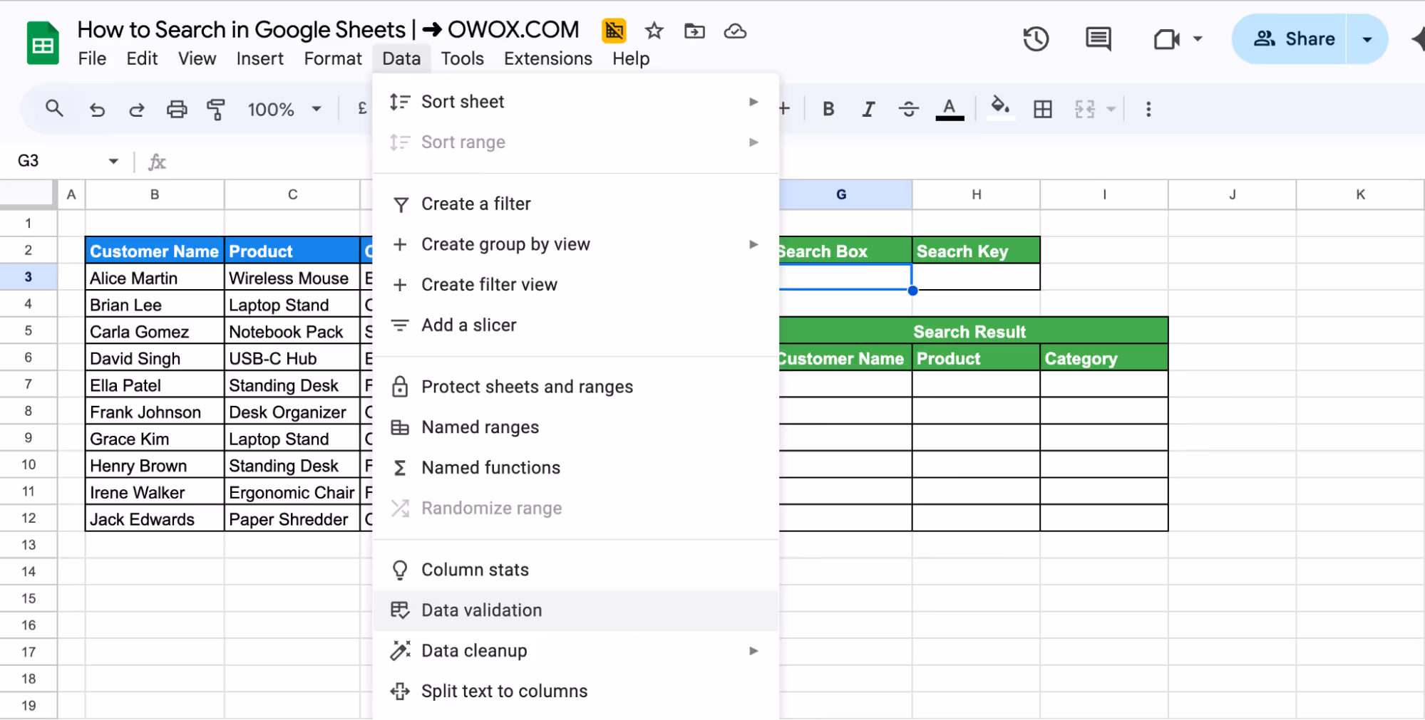
In the Data validation panel, set Criteria to Drop-down, then enter options like Starts With and Contains. Click Done to apply the dropdown in cell G3.

Next, enter a search term in cell H3. Then, click on cell G7 and type the formula below to display results:

=IFERROR(QUERY(B3:D12, "SELECT * WHERE B " & G3 & " '" & H3 & "' "), "No Match")

Here's what each parameter means:

• B3:D12 – The data range with Customer Name, Product, and Category
• B – Tells QUERY to apply the condition to Column B (Customer Name)
• G3 – Pulls the selected search type (like Starts with)
• H3 – Insert the actual search term
• IFERROR(...) – Displays "No Match" if the search returns nothing

This setup allows users to choose how they want to search and instantly view matching results from the dataset, all without using filters or manually scrolling.

Using FILTER and SEARCH Functions for Custom Search

Use the FILTER and SEARCH functions together to create a custom search that returns rows based on partial matches in multiple columns.

First, set up your sheet by assigning cells for filter inputs and a search result table then, manually type your filter values into G4 (Product search) and H4 (Category search).

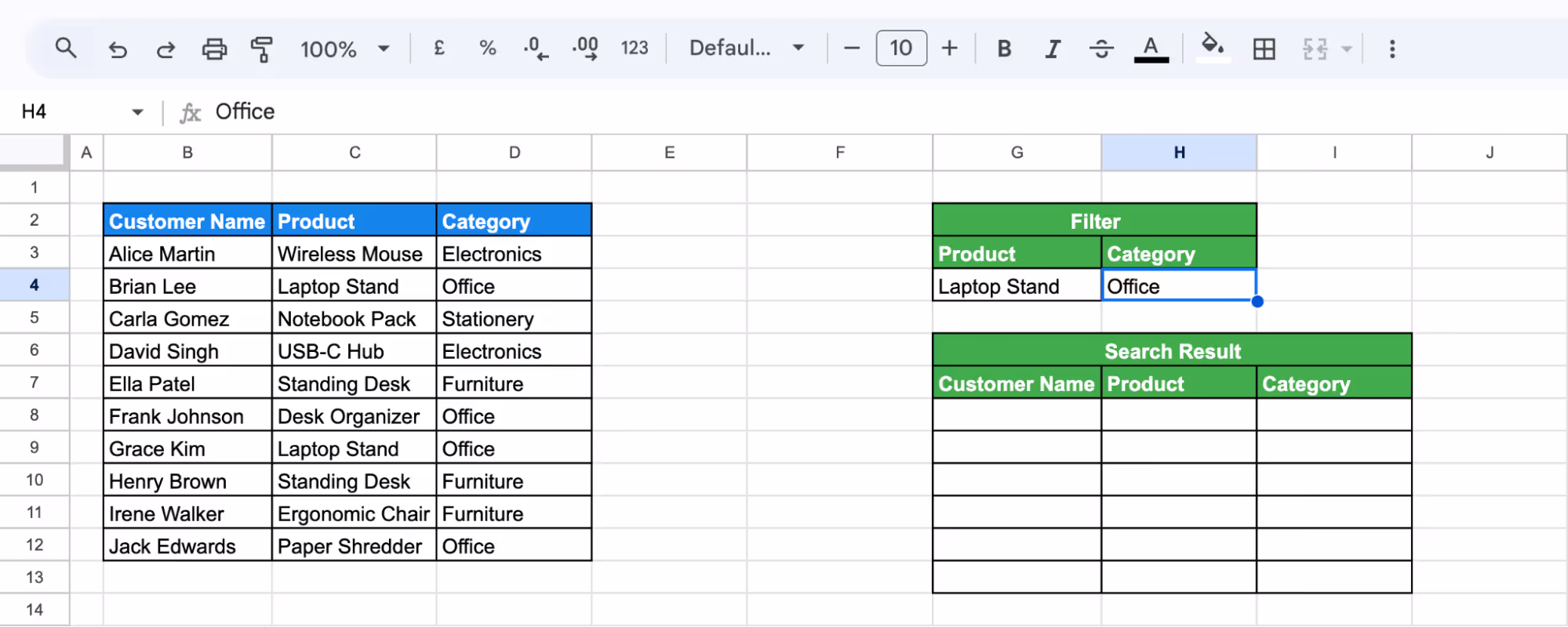
Now, click on cell G8 and enter the formula below:

=IFERROR(FILTER(B3:D12, SEARCH(G4, C3:C12), SEARCH(H4, D3:D12)), "No Match")

Here's what each parameter means:

• SEARCH(G4, C3:C12) looks for the Product search term from cell G4.
• SEARCH(H4, D3:D12) looks for the Category search term from cell H4.
• FILTER(B3:D12, ...) returns rows that match both criteria.
• IFERROR(...) displays "No Match" if there are no results or if cells are left empty.

This setup gives you a simple, flexible way to search by multiple values without complex filtering or scripts.

Searching for a Value’s Position Using the MATCH Function

Use the MATCH function to find the position of a search term within a column. It returns the position of the first match found.

First, assign a cell for the search key and one for the result. In the result cell G4, enter the following formula:

=IFERROR(MATCH(G2, C3:C12, 0), "No Match")

Here's what each parameter means:

• MATCH(G2, C3:C12, 0) searches for the exact value typed in G2 within the Product column (C3:C12) and returns the first match's position.
• IFERROR(...) displays "No Match" if nothing is found or if there’s an error.

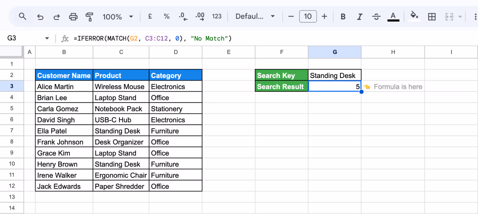
This method is useful when you want to quickly identify where a specific item appears in a list.

Finding the Position of a Substring Using the FIND Function

The FIND function shows the position where a specific character or word first appears within a cell. It's case-sensitive and returns the first match only.

First, assign a cell for the search key (e.g., G2) and one for the result (e.g., G3). Click on G3 and enter the following formula:

=IFERROR(FIND(G2, B12), "No Match")

Here's what each parameter means:

• FIND(G2, B12) checks for the position of the search term in cell B12, which contains a customer name.
• IFERROR(...) prevents errors and shows "No Match" if the term is not found.

This method is handy for pinpointing exactly where a word or character appears in a string, especially when working with text data.

Common Errors and Solutions for Searching in Google Sheets 

Searching in Google Sheets may not always give the results you expect. This section explains common issues and provides simple solutions to help you fix them quickly.

Search Returns No Results Despite Data Being Present

⚠️ Error: If your search shows no matches even though the data is there, it might be hidden, filtered, or have extra spaces that make it unsearchable.

✅ Solution: Unhide all rows and columns, remove any filters, and use the TRIM function to clean up unwanted cell spaces.

Searching for Numbers That Are Formatted as Text

⚠️ Error: If numbers aren’t showing up in search results, they might be stored as text instead of actual numbers, which can stop search tools and formulas from finding them.

✅ Solution: Highlight the cells, go to Format > Number, and set the correct number format. You can also use the VALUE function to convert text to numbers.

Case Sensitivity Affecting Search Results

⚠️ Error: Searches might fail if the "Match case" option is turned on since it will only find results that match the exact uppercase or lowercase letters you typed.

✅ Solution: In the Find and Replace tool, uncheck “Match case” unless you specifically need it. This allows your search to work regardless of the letter case.

Search Not Working Across Multiple Sheets

⚠️ Error: If a search doesn’t work across sheets, the problem might be with incorrect sheet names or broken range references in your formulas.

✅ Solution: Double-check the sheet names and ranges in your formula. Use the INDIRECT function if you want to reference sheet names dynamically or across multiple tabs.

Best Practices for Searching in Google Sheets 

To get better results when searching in Google Sheets, it's useful to follow some basic best practices. These simple tips can help you find the right data faster, avoid common errors, and keep your spreadsheet more organized. Following them will save time and make your work much easier.

Learn Keyboard Shortcuts to Speed Up Search Tasks

Using keyboard shortcuts can help you find data much faster in Google Sheets. For example, pressing Ctrl + F or Ctrl + H opens the search tools right away. These shortcuts save time and reduce clicks, especially when working with large spreadsheets. Learning a few of them can make your work quicker and easier.

Use Descriptive Headers for Faster Identification

Clear and meaningful column headers make it easier to know where to search. Instead of using generic titles like “Data 1” or “Column A,” use names like “Customer Name” or “Invoice Date.” This helps you quickly find the information you need and improves the overall organization of your spreadsheet.

Use Quotation Marks for Exact Match Searches

If you’re looking for an exact word or phrase, putting it in quotation marks can help. This tells Google Sheets to search only for that specific text, not similar or partial matches. Using quotes is especially useful when your data includes similar terms or when accuracy is important in your search.

Enable Regular Expressions for Pattern-Based Searches

For more advanced searching, you can use regular expressions. In the Find and Replace tool, check the option “Search using regular expressions.” This lets you search using patterns, such as finding all cells that start with a certain letter or format. It’s a handy way to filter complex data.

Sort Data Before Searching for Easier Navigation

Sorting your data alphabetically or by number can make searching easier. When data is organized, it’s quicker to scan through results and spot what you’re looking for. You can sort columns using the Data > Sort range option. This small step can save you time during searches.

Restrict Searches to Specific Sheets for Better Accuracy

By default, search tools may scan your entire spreadsheet, including other tabs. To focus your search, click on the specific sheet you want to check before starting. This keeps results more accurate and avoids confusion when working with multiple sheets. It’s a simple way to stay focused on the right data.

💡 Want to work smarter in Sheets as a marketer? Explore OWOX’s guide to essential Google Sheets features, learn how to streamline campaign tracking, automate tasks, and get more insights from your data with less effort.

Advanced Functions to Search and Analyze Data in Google Sheets 

Beyond basic search tools, Google Sheets includes advanced functions that make it easier to locate, filter, and analyze information. These features help users work more efficiently with larger datasets by automating search logic and surfacing results that match specific patterns or criteria.

• CONCATENATE: Combines multiple text strings into one, simplifying the process of merging data from different cells or sources.
• ARRAYFORMULA: Applies a formula to an entire range of cells at once, automating calculations and improving efficiency for large datasets.
• COUNTA: Counts all non-empty cells within a range, making it useful for tracking data entries or identifying missing information.
• HLOOKUP: Searches for a value in the first row of a range and returns a value from the same column in a specified row, ideal for horizontally structured data.
• LOOKUP: Finds the closest match to a search key in a range and returns a corresponding value, useful for retrieving approximate matches in sorted data.
• IF: Returns one value if a condition is true and another if it’s false, enabling logical comparisons and dynamic outputs in your sheets.
• CHAR: Converts a number into a specific character based on the Unicode table, helpful for inserting special characters like line breaks or symbols.

Optimize Your Data Analysis with OWOX: Reports, Charts & Pivots Extension

Making sense of your search results is easier when they’re presented in charts or reports. The OWOX Reports, Charts & Pivots Extension helps you turn spreadsheet data into clear visuals in just a few steps. No complex formulas are needed, which means less time formatting and more time understanding your data.

With OWOX, you can build pivot tables, generate charts, and track key metrics – all directly within Google Sheets. It’s perfect for marketers, analysts, and anyone who wants to turn raw data into insights. Try it out to speed up reporting and decision-making.