A Detailed Guide to SUM, SUMIF, and SUMIFS Functions in Google Sheets

If you work with spreadsheets, whether you're a casual user or a data analyst, becoming comfortable with functions like SUM, SUMIF, and SUMIFS in Google Sheets can significantly help you stay organized, track progress, and demonstrate your impact. The good news? These functions work the same way in Microsoft Excel, too, so once you learn them, you can use them across both platforms.

Whether you’re building reports to monitor your work or performing complex data analysis, these functions allow you to sum data based on various criteria.

In this detailed guide, you’ll learn how to use the SUM function to quickly total data ranges, the SUMIF function to sum data that meets specific criteria, and the SUMIFS function to handle multiple conditions at once. SUM, SUMIF, and SUMIFS are built-in functions so that you can use them right away without any extra setup or coding.

By mastering these tools, you’ll be able to automate your reporting processes, enhance the precision of your data analysis, and extract valuable insights that highlight performance metrics, ultimately leading to a deeper understanding of the overall picture.

Here are some reasons why you should use them:

• Quickly add numbers: The basic SUM quickly adds numbers within a selected cell range, saving time and reducing the potential for manual errors.
• Calculate total value: These functions help you efficiently calculate the total value in a column or range, even as new data is added.
• Handle large datasets: It allows you to calculate totals across multiple cells in a single formula, which is particularly beneficial for handling large datasets.
• Flexibility: The function also offers flexibility by letting you sum single or multiple ranges and seamlessly integrate with other formulas.
• Automatic updates: One helpful feature is that totals update automatically whenever you change or add data, so you don’t have to manually recalculate anything.
• Better accuracy: Learning how to use SUM, SUMIF, and SUMIFS lets you analyze data more accurately, spot patterns more easily, and base your decisions on solid numbers.

Exploring the Basics of SUM Functions in Google Sheets

The SUM function in Google Sheets is a powerful tool for managing data. It allows you to quickly add up ranges of numbers, reducing the risk of manual errors and saving you time. You can quickly calculate the sum of a column in Google Sheets by selecting the entire column or a specific range.

 It also enables you to quickly calculate totals for all the values in a selected range or column. Additionally, you can connect Google Sheets to BigQuery for advanced data analysis.

With the flexibility to sum single or multiple ranges, it ensures dynamic updates as data changes. In the following sections, we’ll cover the basic syntax and provide examples for the SUM, SUMIF, and SUMIFS functions, helping you enhance your data analysis and reporting efficiency.

SUM Function

The SUM function in Google Sheets is a quick way to add up numbers in a range of cells. It simplifies calculations, helps prevent manual errors, and updates the total automatically when the data changes. You can use it to total up an entire column or just a specific group of cells; it all depends on what you're working with.

SUM Function Syntax

The syntax for the SUM function in Google Sheets is:

=SUM(value1, [value2, ...])

Let's break down what these parameters represent:

• value1: The first number or range to sum.
• [value2, ...]: Additional numbers or ranges to include.

You can use ranges (e.g., A1:A10) or individual numbers (e.g., 5, 10) in the formula.

SUM Function Example: How to Sum a Column in Google Sheets

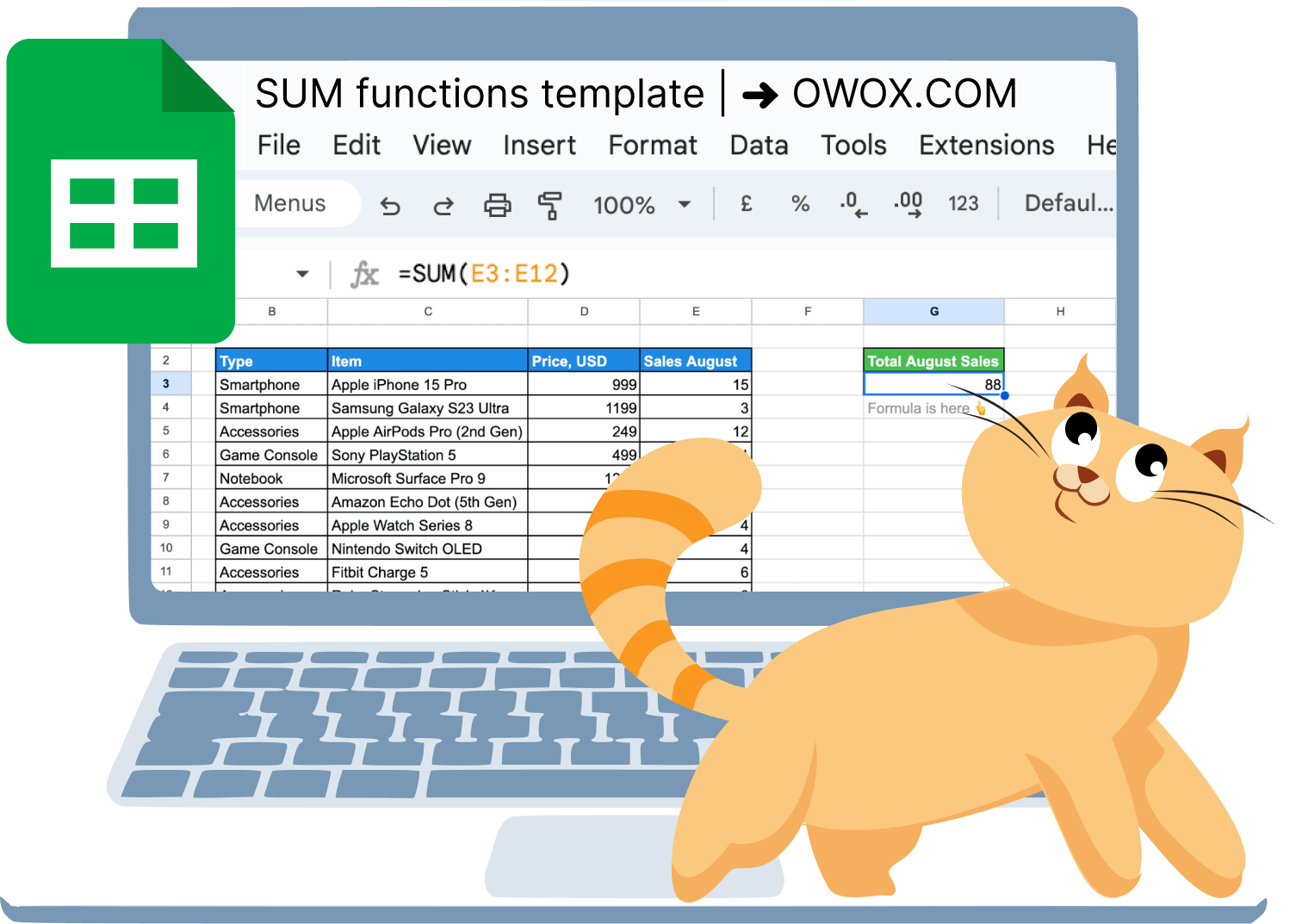
Knowing how to sum a column in Google Sheets helps you quickly calculate totals without writing separate formulas for each row. Let’s say we have a list of the top 10 bestselling gadgets for August and would like to find the total sales in column E.

To calculate the sum of sales data in a column in Google Sheets, you can enter the SUM function manually in a cell. For example, use the following formula:

=SUM(E3:E12)

After typing the formula, press Enter to display the result.

Here’s the breakdown:

• E3:E12: The range in column E where the sales data for the top 10 gadgets is located.

Adjust the range as necessary to match the exact cells where your data is stored.

SUMIF Function

The SUMIF function in Google Sheets adds values based on a specific condition; it is a conditional sum function that allows you to add values only when specific criteria are met. It summarizes data that meets specific criteria, such as totals for items that match a particular label or threshold when you select cells.

SUMIF Function Syntax

The syntax for the SUMIF function in Google Sheets is:

=SUMIF(range, criterion, [sum_range])

Here's the breakdown:

• range: The range of cells to evaluate against the criterion.
• criterion: The condition or criteria to apply.
• [sum_range] (optional): The range of cells to sum if the criterion is met. If omitted, the function sums the range.

SUMIF Function Example: How to Sum a Column in Google Sheets Based on One Condition

Let’s say we have a list of the top 10 bestselling gadgets for August and would like to find the total sales of all accessories in column E.

To calculate the sum of sales data in column E by criterion in cell G3, first make sure you have the cell selected where you want the SUMIF result to appear. Then use the following formula in Google Sheets:

=SUMIF(B3:B12, G3, E3:E12)

Here’s the breakdown:

• B3:B12: The range of cells to evaluate against the criterion.
• G3: The criteria to apply, “Accessories”
• E3:E12: The range of cells to sum.

💡 The IF function is essential for making decisions in your spreadsheets based on specific conditions. Explore our comprehensive guide on the IF function to streamline your data processing and enhance decision-making in Google Sheets.

SUMIFS Function

The SUMIFS function in Google Sheets sums values based on multiple criteria, allowing you to specify different conditions across various ranges to get a total that meets all the selected criteria. 

You can use SUMIFS to sum values across multiple columns in Google Sheets by applying criteria to different columns. This makes it ideal for reports that consolidate totals from multiple columns, like monthly performance or product category groupings.

SUMIFS Function Syntax

The syntax for the SUMIFS function is:

=SUMIFS(sum_range, criteria_range1, criterion1, [criteria_range2, criterion2, ...])

Let's break it down:

• sum_range: The range of cells to sum.
• criteria_range1: The range to apply the first criterion.
• criterion1: The condition for the first criteria range.
• [criteria_range2, criterion2, ...] (optional): Additional ranges and criteria.

💡 While SUMIF, and SUMIFS help with conditional sums, the IFS function is perfect for complex conditional calculations. Dive into our detailed guide on the IFS function to enhance your spreadsheet decision-making capabilities.

SUMIFS Function Example: How to Sum a Column in Google Sheets with Multiple Conditions

Let’s say we have a list of the top 10 bestselling gadgets for August and would like to find out the sum of the sales of accessories with prices above $200 in column E.

=SUMIFS(E3:E12, B3:B12, G3, D3:D12, ">200")

Let’s explain the formula:

• E3:E12: The range of cells containing the sales figures you want to sum.
• B3:B12: The range where the value should match the one in G3.
• G3: The specific value used to filter B3:B12.
• D3:D12: the range where the condition “>200” is applied.
• “>200”: The criterion indicating that the values in D3:D12 should be greater than $200.

If you use a full-column range like E: E in your SUMIFS formula, it will automatically pick up any new entries added to that column. This keeps your totals current without needing to update the formula every time you add data.

Practical Examples of Using SUM Functions

The SUM functions are flexible and helpful in various everyday tasks. You can use them to total up values in a column, add all the numbers in a selected range, or have your totals update automatically as your data grows or changes.

Master SUM Functions With Our Practical Template!

Uncover the power of SUM, SUMIF, and SUMIFS functions to enhance your data management. Explore practical examples to see how these functions simplify complex calculations, automate reporting, and drive insightful analysis.

Claim your FREE template today!

Using SUM to Add Cell Values in a Column

Adding up values in a column with the SUM function is one of the basics of working with data in Google Sheets. It only counts numerical entries, so it skips over any text or empty cells. This makes it a reliable way to total up numbers within a specific range, useful for tasks such as financial summaries, inventory tracking, or analyzing survey data.

Example:
Let’s say you want to calculate total sales for items sold in August:

=SUM(E3:E12)

This function saves time and reduces the risk of manual errors associated with manually adding numbers. It dynamically updates the total value if the numeric values in the range change, ensuring that your calculations remain accurate and up-to-date.

Using SUM to Add Cell Values in a Row

Using SUM to add cell values in a row enables you to total numbers across a horizontal range quickly. You can sum a selected range or selected cells in a row.

For example, we have sales data for June, July, and August. We can calculate the total summer sales by applying the following formula:

=SUM(E3:G3)

Additionally, dragging it down will provide us with the summer sales totals for all items. To copy the SUM down a column, you can double-click the small blue box in the bottom right corner of the function cell, which will automatically apply the formula to the remaining rows in the column.

Using SUM to Add Cell Values in Non-adjacent Cells

Using the SUM function to add values in non-adjacent cells allows you to sum up specific numbers scattered across your spreadsheet. Instead of summing a continuous range, you can select individual cells or ranges by separating them with commas. You can also apply this method when your data spans multiple columns and you want to add only certain values selectively.

Let’s say we want to total the sales of Apple items during the summer. We can select only the cells with sales data for iPhones, AirPods, and Apple Watches:

=SUM(E3, F3, G3, E5, F5, G5, E9, F9, G9)

This flexibility is beneficial when your data isn’t in a single block, enabling precise calculations without rearranging your spreadsheet layout.

Applying the SUM Function across Sheets

Applying the function across multiple sheets in Google Sheets allows you to total values from the same cell range across different tabs. This is particularly useful when consolidating data from multiple categories or periods.

For example, we have sales data from the store for July and August in two different sheets, named 'Sales July' and 'Sales August', that are summed up.

To calculate the total, let's use this formula:

=SUM('Sales July'!G3, 'Sales August'!G3)

This approach simplifies calculations, ensuring that all relevant columns from different Google Sheets data sheets are included in the final total.

How to Quickly Sum in Google Sheets without Any Formulas

You can quickly sum values in Google Sheets without using any formulas by simply selecting the range of cells you want to add. As you select the cells, Google Sheets will automatically display the sum in the bottom-right corner of the screen, along with other basic statistics, such as the average and count.

Alternatively, you can use the menu bar or functions menu to access the function: simply select your desired range, then click on the Greek letter sigma (Σ) in the toolbar or open the dropdown menu to choose SUM and quickly calculate the total.

Another option is to just highlight the cells you need using your mouse or trackpad before typing in the formula or choosing it from the menu.

This feature is ideal for quickly obtaining a total without the need to enter a formula, making it a convenient tool for fast calculations during data reviews or when working with temporary datasets.

Advanced Applications of SUMIF and SUMIFS in Google Sheets

Explore advanced applications of SUMIF and SUMIFS in Google Sheets, including exact text matches, wildcard characters, date-based criteria, and logical operators. Master these techniques for precise and efficient data analysis.

SUMIF with Exact Text Match Criteria

Using SUMIF with exact text match criteria allows you to sum values based on cells that exactly match a specified text. For example, we would like to find out the sales of game consoles in August. Let's use the formula:

=SUMIF(B3:B12, "Game Console", E3:E12)

This method is useful for aggregating data where precise text matching is required, such as calculating total sales for a specific product or summarizing data based on exact labels or categories.

SUMIF Using Wildcard Characters for Partial Text Match

Using wildcard characters with the SUMIF function allows you to sum values based on partial text matches. Wildcards are useful for matching patterns rather than exact text.

Let's calculate the total number of Apple items we sold in August.

Let's apply the following formula for it:

=SUMIF(C3:C12, "*Apple*", E3:E12)

The asterisk * works as a wildcard, matching any number of characters. It’s useful when you want to group data with slight differences in text, for example, adding up sales for items that include a certain keyword.

SUMIF Formulas for Date-based Criteria

SUMIF formulas for date-based criteria allow you to sum values based on specific dates or date ranges.

For example, to calculate all sales summaries before August 15th, 2024, you can use the criterion as follows:

=SUMIF(F3:F12, "<15/08/2024", E3:E12)

If you need to sum cells conditionally based on today's date, you can incorporate the TODAY() function into your criterion argument.

We need to review all sales summaries from the past 20 days due to current sales dynamics. To achieve this, we should identify summaries dated more than 20 days ago that include only numerical values.

And reflect this in the formula:

=SUMIF(F3:F12, ">" & TODAY() - 20, E3:E12)

This approach is essential for summarizing data within specific periods, as well as monthly or yearly totals.

SUMIF with Multiple Criteria Using OR Logic

SUMIF with multiple criteria using OR logic allows you to sum values that meet at least one of several conditions.

For instance, if we want to calculate the sales of smartphones and accessories, this can be achieved using the following conditions:

=SUMIF(B3:B12, "Smartphone", E3:E12) + SUMIF(B3:B12, "Accessories", E3:E12)

This approach combines multiple SUMIF functions to handle scenarios where you need to sum data based on different, non-overlapping criteria.

Using SUMIF and SUMIFS with Logical Operators

Using SUMIF and SUMIFS with logical operators enhances your ability to sum values based on complex conditions.

Here is a list of logical operators you can use:

• - Greater than - >
• - Less than - <
• - Equal to - =
• - Greater than or equal to - >=
• - Less than or equal to - <=
• - Except for - <>

The main difference between SUMIF and SUMIFS comes down to how many conditions you're working with. SUMIF is great when you only need to filter based on one rule, but if you have more than one condition, like filtering by both category and date, SUMIFS is the better choice.

In short, use SUMIF for simple, single-condition cases, and SUMIFS when things become a bit more specific. For the first example, we'd like to find the number of sales of items priced over $500.

To do this, let's apply the following formula:

=SUMIF(D3:D12, ">500", E3:E12)

For storage optimization, let's determine if we have sales of items priced over $500 with fewer than 5 units sold. We want to count the number of such sales to decide if we should continue stocking these items.

Let's reflect it in the formula:

=SUMIFS(E3:E12, D3:D12, ">500", E3:E12, "<5")

Logical operators help refine criteria for more precise calculations, enabling you to efficiently handle a variety of conditions and exclusions.

Applying SUMIF and SUMIFS with Empty or Non-empty Cells

Applying SUMIF and SUMIFS with empty or non-empty cells allows you to sum values based on whether a particular cell range is blank or contains data. When using SUMIF or SUMIFS, an empty cell is treated as zero in calculations, and you can use an empty cell as a criterion to filter data.

 This is useful for filtering out incomplete records or focusing on specific entries. In these examples, we can use SUMIFS to handle both empty and non-empty cells with multiple conditions, whereas SUMIF is sufficient when the condition is simplified to just one.

Let’s say we have some missing data in the store due to price changes in August. We need to calculate the number of items with missing price data.

To do this, let’s use the following formula:

=SUMIF(D3:D12, "", E3:E12)

For multiple conditions, let’s suppose we have blank data cells regarding item prices and sold items due to a worker’s mistake. We need to determine the number of complete operations, excluding those with missing data. 

This formula adds up the sales in August for items where both the price and sales data are available, effectively excluding any rows with missing information:

=SUMIFS(E3:E12, C3:C12, "<>", D3:D12, "<>")

These functions help streamline data analysis by letting you target specific conditions, such as summing only completed transactions or identifying missing information.

Using SUMIFS to Sum Cells with Multiple AND Conditions

Using the SUMIFS function, you can sum cells that meet multiple conditions simultaneously.

We want to count the number of Apple accessories sold in quantities greater than 1.

Let's apply this formula:

=SUMIFS(E3:E12, B3:B12, "Accessories", C3:C12, "*apple*", E3:E12, ">1")

The SUMIFS function allows you to apply both conditions in one formula, ensuring that only the data meeting both criteria is included in the total. This is particularly useful for analyzing specific subsets of your data.

Combining SUM Functions with Other Google Sheet Functions

If you’re working with large datasets or dynamic criteria, Google Sheets supports advanced summation methods using functions like FILTER, ARRAYFORMULA, and logical conditions.

Combining SUM and FILTER Functions

Combining the SUM and FILTER functions in Google Sheets allows you to sum only the values that meet specific criteria. The FILTER function narrows down the dataset to include only the rows that match your conditions, and the SUM function then calculates the total of those filtered values.

 This is particularly useful when you want to sum data from a large dataset based on dynamic conditions. We want to sum the sales in August for items priced over $500.

Apply the formula:

=SUM(FILTER(E3:E12, D3:D12 > 500))

This formula will return the total sales in August for all items priced over $500, based on the data in your table.

SUM with ARRAYFORMULA to Sum Multiple Rows

Using the SUM function in Google Sheets allows you to sum values across multiple rows or columns in a single formula. ARRAYFORMULA enables operations to be applied across an entire range of cells, making it efficient when dealing with large datasets or when you want to perform the same calculation across multiple rows or columns.

 Let's use ARRAYFORMULA combined with a multiplication operation to calculate the total amount of money generated from sales. By multiplying the price of each item by the number of units sold, we can then sum the results to get the total revenue.

Let's use the formula:

=ARRAYFORMULA(SUM(D3:D12 * E3:E12))

This technique also works when summing values spread across multiple columns, such as monthly sales, regional splits, or category totals.

Using SUMIF with FIND and ARRAYFORMULA for Case-sensitivity

The SUMIF function in Google Sheets is not case-sensitive by default. However, you can combine SUMIF with FIND and ARRAYFORMULA to perform a case-sensitive sum.

The FIND function is case-sensitive, meaning it distinguishes between uppercase and lowercase letters. By using it within an ARRAYFORMULA, you can create a case-sensitive condition for summing values.

Suppose you have a list of items with varying cases, and you want to sum the sales figures only for the exact case-sensitive match of the item "Apple" (not "apple" or "APPLE").

Let's apply the formula:

=SUMIF(ARRAYFORMULA(FIND("Apple", C3:C7)), ">0", E3:E7)

Here's the breakdown:

• FIND("Apple", C3:C7): searches for the substring "Apple" in each cell within the range C3:C7. It returns the position of the substring if found and an error if not found. This function is case-sensitive.
• ARRAYFORMULA(...): ensures that FIND is applied to each cell in the range C3:C7.
• SUMIF(..., ">0", E3:E7): sums the values in E3:E7 (Sales August) where the result of FIND is greater than 0 (meaning the exact substring "Apple" was found).

This formula will return the sum of sales for items that exactly match "Apple" with the correct case, ignoring any other variations, such as "apple" or "APPLE".

Combining SUMIFS with TODAY Function

The SUMIFS function can be combined with the TODAY function to sum values based on date criteria that involve the current date. This is particularly useful when you want to analyze data in real-time or track ongoing trends, such as sales made today, this week, or within a specific time range relative to the current day.

Assume we have a sales record, and we want to calculate the total sales of items sold today.

Let's reflect on it in this formula:

=SUMIFS(E3:E7, F3:F7, TODAY())

This is useful when tracking performance by date across a specific column in Google Sheets that holds timestamped records.

Addressing Common Pitfalls with SUM Functions and How to Avoid Them

Learn how to troubleshoot and avoid common issues with SUM functions, including syntax errors, incorrect references, circular dependencies, data type mismatches, and handling hidden or filtered rows.

Syntax Error in SUM Formula

⚠️ Error: Incorrectly written SUM formula due to missing or extra parentheses, commas, or incorrect syntax.

Example of an error with a missing closing parenthesis

=SUM(E3, E5, E7

Another example with a missing comma between E5 and E7:

Solution: Ensure all opening parentheses have corresponding closing parentheses. Use commas to separate individual arguments or cell ranges within the function. Confirm that the function name and arguments follow Google Sheets syntax rules.

Cells Not Recognized as Numbers

⚠️ Error: If your cells are formatted as text, the SUM function might not work as expected. It won’t add those values, which can lead to incorrect or missing totals. Ensure the cells are set to the “Number” format so the function can perform its job properly.

✅ Solution: To make sure the SUM function works the way it should, it's important that all the data you're adding up is actually recognized as numbers. 

Here’s how to check:

• Set the Right Format: Select your cells, go to the toolbar, click on the “123” (More formats) button, and choose “Number.” This instructs Google Sheets to treat those values as actual numbers, rather than text.
• Watch Out for Auto-Formatting: Sometimes, when a cell is set to “Automatic,” numbers can be misinterpreted as text. If your total seems off, switch the format to “Number” manually just to be safe.
• Linked Data Matters Too: If your formula is pulling data from another range, ensure that range is also formatted as “Number”. Otherwise, even well-written formulas can break or return the wrong total.

Incorrect Cell References in SUM Function

⚠️ Error: Incorrect cell references can lead to incorrect totals when using the SUM function. This issue arises if the formula includes the wrong cells or an unintended range of cells.

✅ Solution: Ensure that the SUM function is pointing to the correct column in Google Sheets, row, or range of cells to avoid incorrect totals. It may seem obvious, but it's a common mistake to overlook, especially when working quickly on a project.

Circular Dependency Detected in SUM Calculation

⚠️ Error: Circular dependency in a SUM calculation occurs when the formula refers to its cell either directly or indirectly, creating a loop that prevents proper calculation.

✅ Solution: Identify and remove the circular reference by checking the formula to ensure it does not include its cell or range. You may need to adjust the formula or use different cells to avoid the loop. To help with this, sheets often provide a warning or error message indicating a circular dependency, which can guide you in resolving the issue.

Formula Errors in SUM Range

When summing a column that includes formulas, if any formula within that column results in an error, the SUM function will also display the same error.

This can lead to confusion, making it seem as though there's a problem with the function itself, when in fact, the issue lies with one of the formulas within the sum range.

⚠️ Error: If there are broken or invalid formulas in the cells you’re trying to sum, the function might return the wrong result or none at all.

✅ Solution: Check the SUM formula for any invalid references or incorrect syntax. Ensure that all cell ranges are valid and properly formatted. For example, verify that the cell range specified exists and contains numbers or valid data. If errors persist, use error-checking tools in Google Sheets, such as IFERROR function, to identify and correct the issues in the formula.

SUM Ignoring Hidden or Filtered Rows

⚠️ Error: If you have hidden rows in your spreadsheet, the SUM function might produce unexpected results. Although the formula itself calculates correctly, it can give a larger total than anticipated by including numbers from hidden rows that aren't visible.

✅ Solution: If you need to include hidden or filtered rows in your sum, use the SUBTOTAL function instead of SUM. The SUBTOTAL function can handle filtered data and provides options to include or exclude hidden rows based on your needs. Code 109 in the SUBTOTAL(function_code, range) function calculates the sum of a range while ignoring any values in hidden rows.

Mismatched Range Sizes in SUMIF and SUMIFS (Google Sheets)

⚠️ Error: Mismatched range sizes in SUMIF or SUMIFS occur when the ranges specified for criteria and sum do not have the same number of cells, leading to errors or incorrect calculations.

✅ Solution: Make sure the range you're applying the condition to and the range you're summing have the same number of rows (or columns, if you're working horizontally). If they don’t line up, the function might not return the right result; just double-check and adjust the ranges so they match.

Incorrect Criteria Syntax in SUMIF

⚠️ Error: If your SUMIF formula isn’t giving the right result or shows an error, it might be due to how the criteria are written. This often happens when quotes are missing, characters are misplaced, or the format just doesn’t match what the formula expects.

✅ Solution: Ensure that the criteria are properly enclosed in quotes for text or formatted correctly for numeric comparisons. Double-check for typos and ensure that the criteria are specific and correctly structured.

Data Type Mismatch in SUMIF

⚠️ Error: A mismatch between the type of data in your range and the criteria you're using can throw off your SUMIF. For example, if your range contains numbers but your criteria are treated as text, the function might not work the way you expect.

✅ Solution: Make sure text criteria are inside quotes, and that number comparisons (like ">100") are correctly formatted. It's also a good idea to check for typos or extra spaces that can break the formula.

Best Practices and Tips for Using the SUMIF Function Efficiently

Learning how to use the SUMIF function well can streamline your work in Google Sheets. It's great for adding up values that meet a specific condition, whether that's a certain category, keyword, or number. Ensure you use the correct syntax, particularly when working with case-sensitive text or custom criteria.

Tip: Be aware of merged cells or non-numeric data in your range. They can skew your results or prevent the function from working as expected. Always double-check your data format and structure to ensure accurate results.

Use SUMIF for Single Conditions Only

The SUMIF function is designed to sum values based on a single criterion, making it an ideal choice when you need to filter data by one specific condition. Here's an example of the SUMIF function, which allows for only one range, one criterion, and one sum_range.

Remember that SUMIF Ignores Case Sensitivity

SUMIF itself is case-insensitive. To create a case-sensitive SUMIF formula that distinguishes between uppercase and lowercase characters, combine SUMIF with ARRAYFORMULA and FIND, as demonstrated in this example.

Follow the Correct Syntax for SUMIF Criteria

To ensure your Google Sheets SUMIF formula works correctly, it's essential to express the criteria properly.

When the criterion includes text, a wildcard character, or a logical operator followed by a number, text, or date, enclose the criterion in quotation marks.

For example:

• =SUMIF(A2:A10, "Apple", B2:B10)
• =SUMIF(A2:A10, "*", B2:B10)
• =SUMIF(A2:A10, ">5")
• =SUMIF(A5:A10, "<>Apple", B5:B10)

If the criterion involves a logical operator combined with a cell reference or another function, use quotation marks to start the text string and an ampersand (&) to concatenate and complete the string.

For example:

• =SUMIF(A2:A10, ">"&B2)
• =SUMIF(A2:A10, ">"&TODAY(), B2:B10)

When using SUMIF, ensure that:

• Text criteria are enclosed in quotes.
• Wildcards are appropriately used when partial matches are needed.
• Logical operators are used correctly for numeric comparisons.
• Cell references can replace text or number criteria for dynamic calculations.

Essential Google Sheets Formulas for Advanced Data Analysis

Google Sheets comes with a range of useful formulas that make working with data easier and more efficient. Here’s a quick look at some of the key ones and how they can help:

• VLOOKUP: Searches for a value in the first column of a range and returns a matching value from another column in the same row.
• UNIQUE: Pulls out only the distinct values in a range, removing any duplicates.
• Pivot Tables: Ideal for summarizing and reorganizing large datasets, making analysis and reporting more straightforward.
• MATCH: Locates and returns the position of a specific item within a range, useful for indexing.
• COUNT and COUNTA: COUNT adds up the number of cells that contain numbers, while COUNTA counts everything that’s not empty.
• INDEX and MATCH: This combo gives you a more flexible way to look up values compared to VLOOKUP, especially when your data isn’t structured in a way that VLOOKUP expects.
• AVERAGE: Calculates the mean of a set of numbers, ideal for finding central tendencies in data sets.

Create Dynamic Pivots and Visualize Data with OWOX: Reports, Charts & Pivots Extension

Easily create dynamic pivots and visualize data by integrating BigQuery with Google Sheets using the OWOX: Reports, Charts & Pivots Extension. Simplify data management, automate imports, and gain powerful insights for informed decision-making!