How to link cells, tabs and spreadsheets in Google Sheets
Reference a cell on another tab with ='Sheet2'!A1, pull matching values with VLOOKUP, combine tabs with QUERY and FILTER, connect two spreadsheet files with IMPORTRANGE, and add clickable links between tabs. With examples and fixes for the errors that linking produces.

To link a cell from another tab in Google Sheets, type an equals sign, the tab name, an exclamation mark and the cell: =‘Sheet2’!A1. The cell then shows whatever is in A1 of Sheet2 and follows it when it changes. To link data from a different spreadsheet file, use IMPORTRANGE. To make a clickable link that jumps to another tab, use Insert → Link.
| You want to | Use |
|---|---|
| Show a cell or range from another tab | ='Sheet2'!A1 or ='Sheet2'!A1:C10 |
| Pull the matching value for an ID from another tab | VLOOKUP |
| Combine or filter rows from other tabs | QUERY, FILTER, curly braces |
| Bring in data from another spreadsheet file | IMPORTRANGE |
| Jump to another tab or range with a click | Insert → Link |
The examples below use two tabs of one spreadsheet.
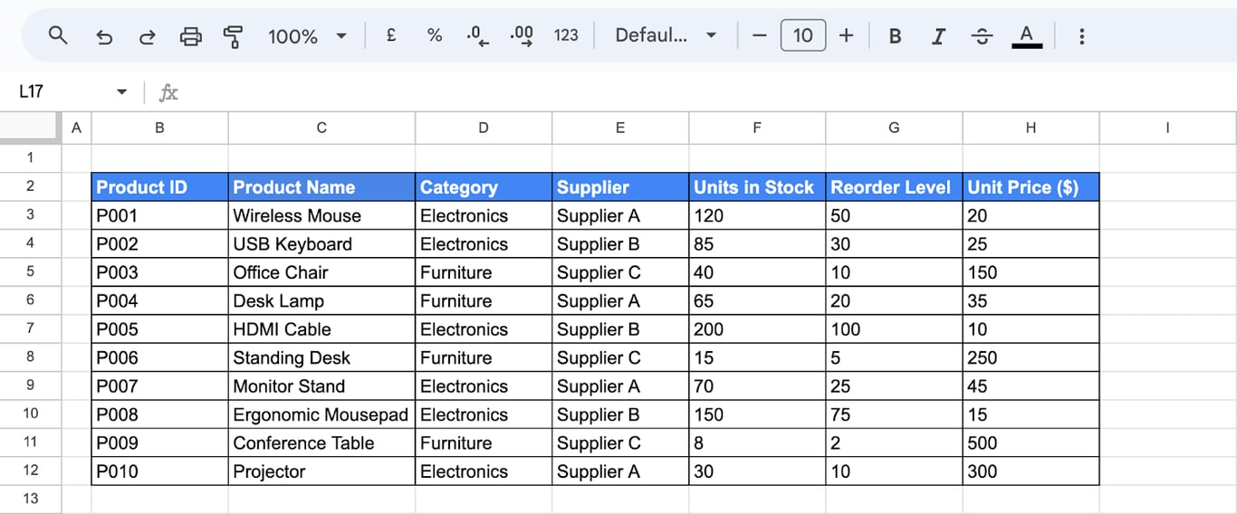
Inventory Management lists the products in stock: product ID, name, category, supplier, units in stock, reorder level and unit price.
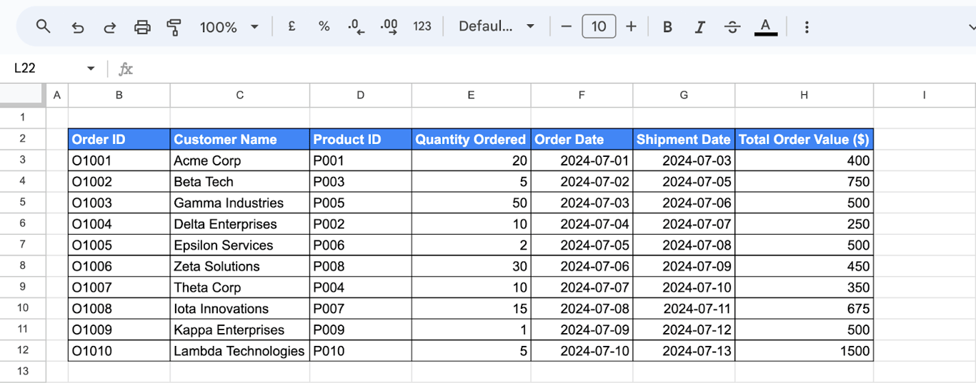
Sales Orders lists the orders: order ID, customer name, product ID, quantity ordered, order date, shipment date and total order value.
Reference a cell or a range on another tab
Reference a cell or a range on another tab
One cell
='SheetName'!CellReference
The single quotes are required when the tab name contains a space, and harmless when it does not. To show cell B3 of the Inventory Management tab on another tab:
='Inventory Management'!B3
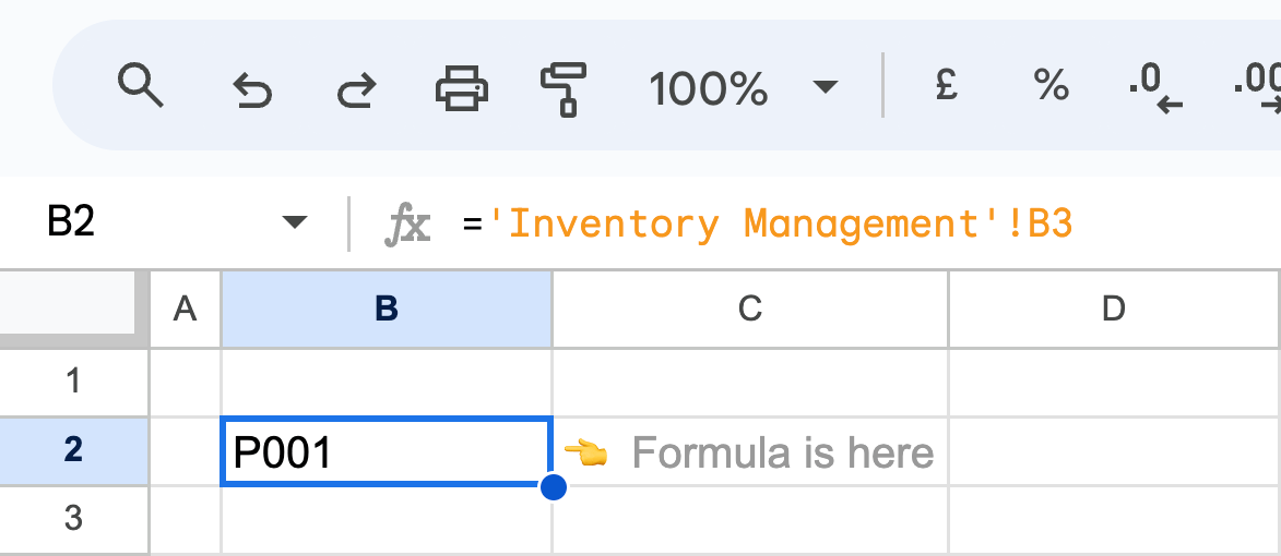
You do not have to type the reference. Type =, click the other tab, click the cell and press Enter; Google Sheets writes the reference for you.
A range
The same syntax takes a range. This shows the customer names from the Sales Orders tab:
='Sales Orders'!C2:C11
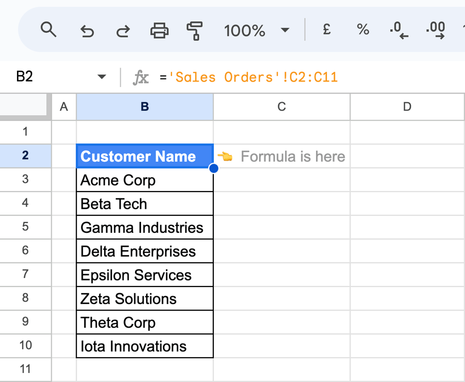
The values fill the cells below the formula, so those cells must be empty.
A range inside a function
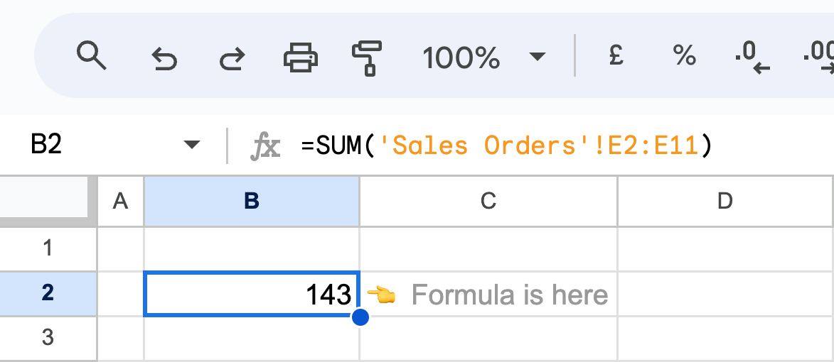
A reference to another tab works anywhere a normal reference does. To total the quantities ordered:
=SUM('Sales Orders'!E2:E11)
Look up matching values from another tab
Look up matching values from another tab
A plain reference copies cells by position. When you need the value that belongs to a particular ID, use a lookup.
VLOOKUP
=VLOOKUP(search_key, range, index, [is_sorted])
- search_key: the value to look for.
- range: the table to search. The key is looked up in its first column.
- index: the number of the column to return, counting from the first column of the range.
- is_sorted (optional): FALSE (or 0) for an exact match, which is what you want for IDs.
To get the unit price of a product by its ID from the Inventory Management tab:
=VLOOKUP('Inventory Management'!B3,'Inventory Management'!$B$3:$H$12,7,0)
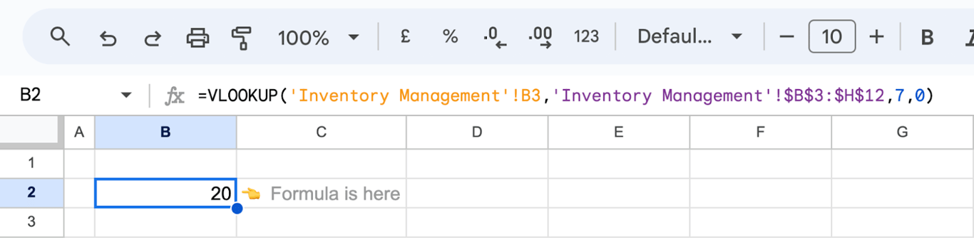
The formula looks up the product ID in the first column of B3:H12 and returns the value from the seventh column, the unit price. The dollar signs keep the table fixed when the formula is copied down.
💡 More on lookups in our guide to VLOOKUP in Google Sheets.

HLOOKUP
HLOOKUP does the same for data laid out in rows: it searches the first row of the range and returns a value from the row you name.
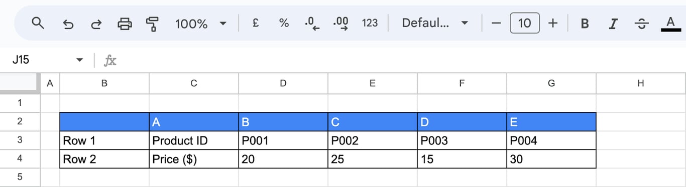
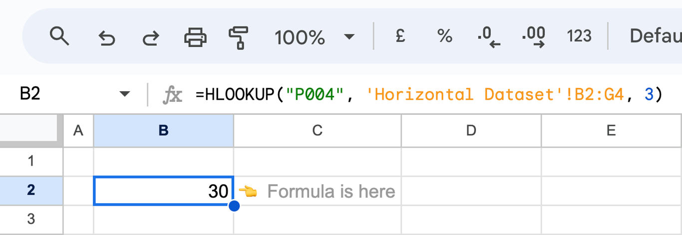
To find the value for product P004 in the third row of this table:
=HLOOKUP("P004", 'Horizontal Dataset'!B2:G4, 3)
INDIRECT: a reference built from text
=INDIRECT(cell_reference_as_string, [is_A1_notation])
INDIRECT turns a text string into a reference. That lets you build the tab name or the range from the contents of other cells, for example to switch between monthly tabs with a drop-down.
=INDIRECT("'Inventory Management'!C4:C10")
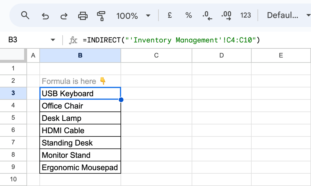
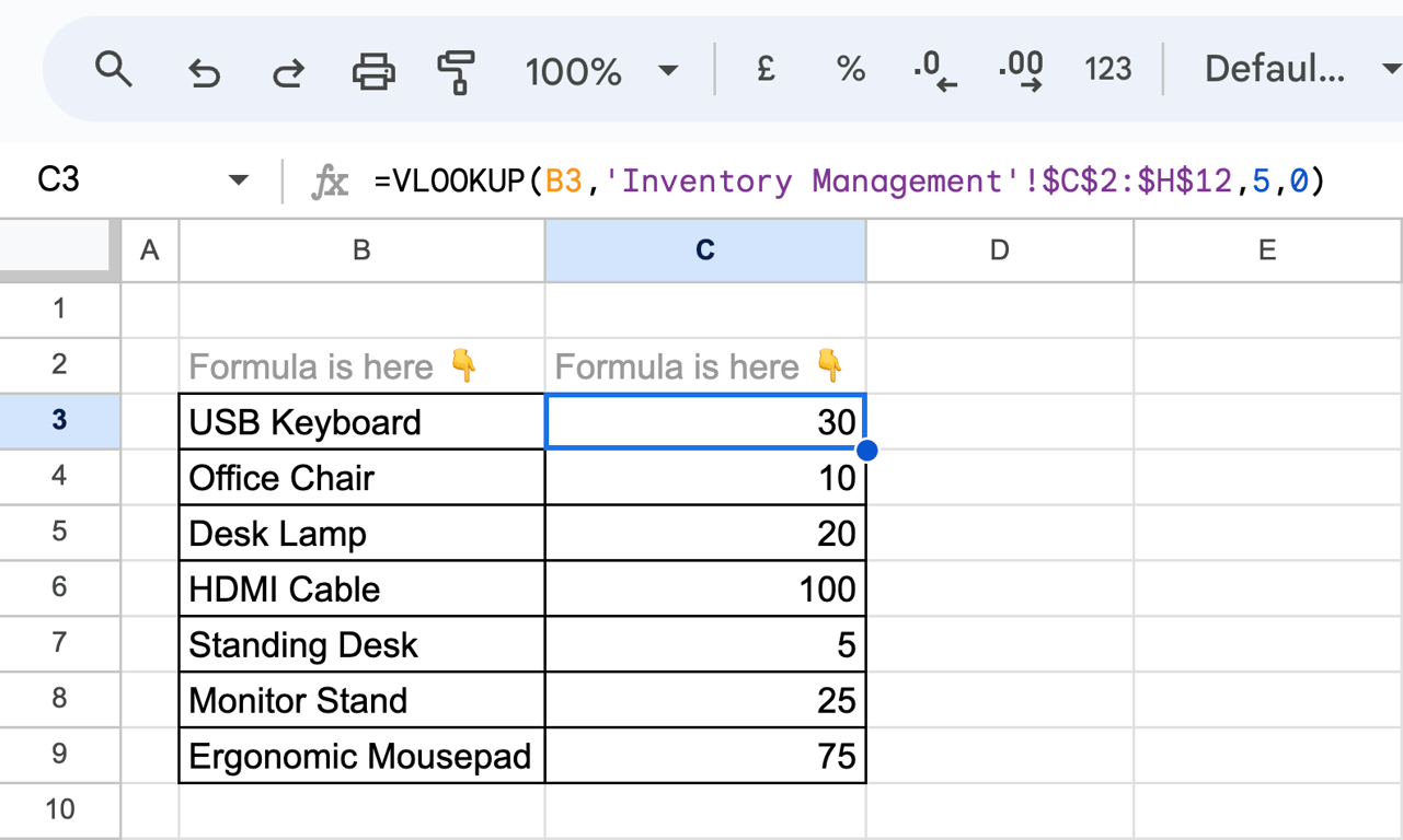
The result is the product names in C4:C10. With the names in place, a VLOOKUP returns the reorder level of each product:
=VLOOKUP(B3,'Inventory Management'!$C$2:$H$12,5,0)
One caution: a reference inside INDIRECT is text. If the tab is renamed, a normal reference updates itself and an INDIRECT string does not.
OWOX Data Marts
See your first report built in real time. 15 minutes.
- Connect your data warehouse
- Pick your metrics
- Get a live Google Sheets report
In the time it takes to write a ticket. Then imagine never writing that ticket again.
Book a DemoWe'll use your actual use case
Combine and filter data from other tabs
Combine and filter data from other tabs
Two ranges side by side with QUERY
Curly braces build an array out of several ranges: a comma puts them side by side, a semicolon stacks them one under the other. QUERY can then filter the combined array.
=QUERY({'Inventory Management'!B2:G11, 'Sales Orders'!B2:G11}, "select * where Col1 <> ''", 1)
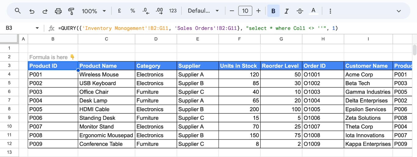
- {Range1, Range2}: places the two ranges next to each other. Both must have the same number of rows.
- select * where Col1 <> ‘’: returns every column, for the rows where the first column is not empty. Inside an array, columns are called Col1, Col2 and so on.
- 1: the first row is a header.

Rows that meet a condition with FILTER
The FILTER function returns the rows of a range that pass a test:
=FILTER(range, condition1, [condition2, …])
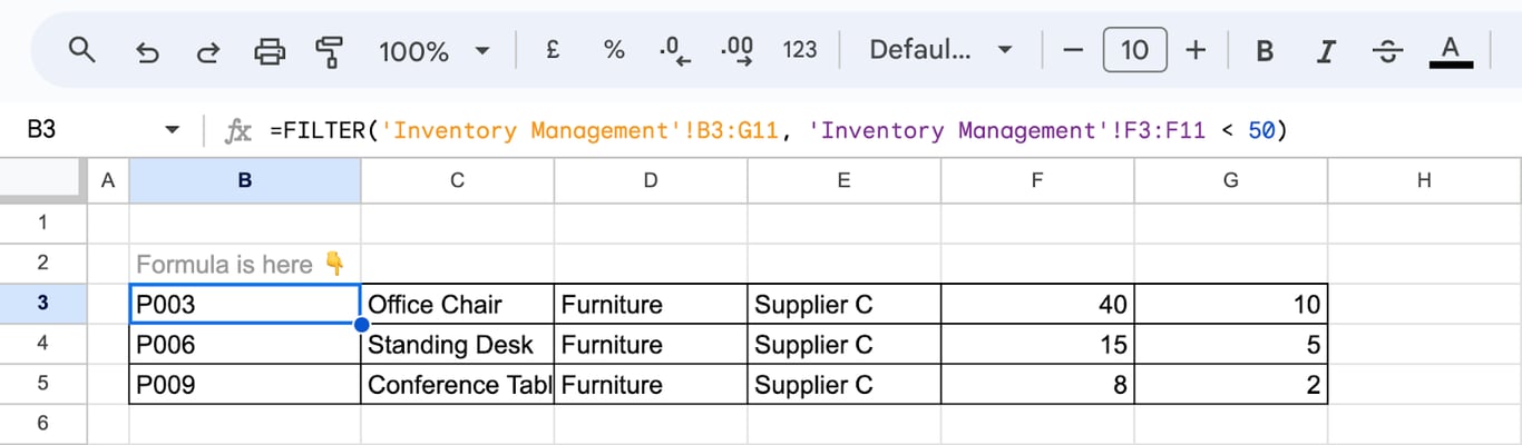
To list the products with fewer than 50 units in stock:
=FILTER('Inventory Management'!B3:G11, 'Inventory Management'!F3:F11 < 50)
Several tabs stacked into one column
Semicolons stack the results. This puts a heading, the product IDs from one tab and the order IDs from the other into a single column:
={
"Pulling Data from Multiple Sheets into One Column";
 FILTER('Inventory Management'!B2:B, LEN('Inventory Management'!B2:B) > 0); FILTER('Sales Orders'!B2:B, LEN('Sales Orders'!B2:B) > 0)
}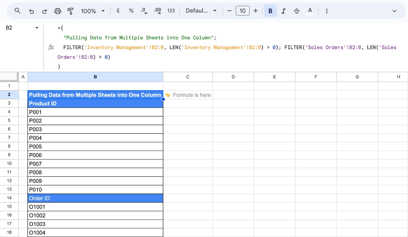
The LEN test leaves out the empty cells at the bottom of each open-ended range.
Whole columns or rows
To mirror entire columns of another tab, reference the columns without row numbers:
={'Inventory Management'!B:D}
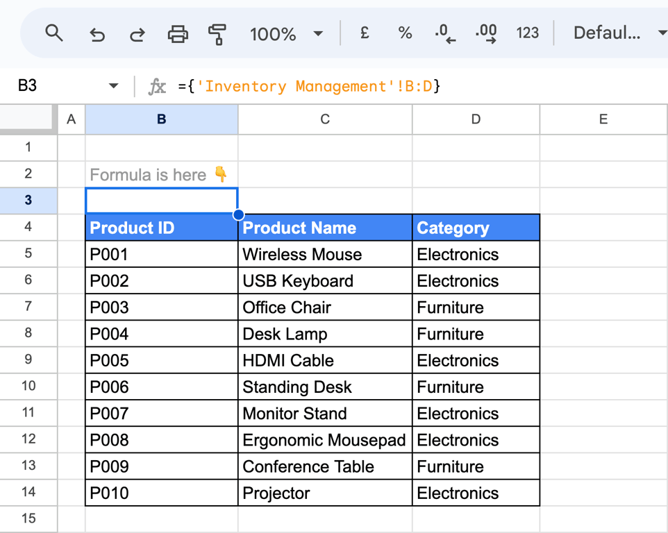
And for entire rows, reference the row numbers:
={'Inventory Management'!2:5}
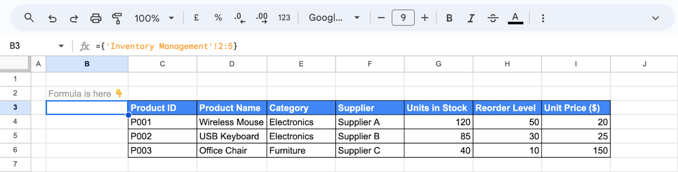
Jump to another tab with a clickable link
Jump to another tab with a clickable link
A link does not copy data. It takes the reader to a place in the spreadsheet, which is useful for a table of contents or a “see details” cell.
- Select the cell that should hold the link.
- Go to Insert → Link (Ctrl + K, or Cmd + K on a Mac).
- Choose Sheets and named ranges.
- Pick a tab, or choose Select a range of cells to link and enter the range, for example ‘Inventory Management’!C2:C12.
- Click Apply.
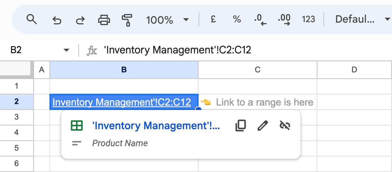
Link to a named range
A named range gives the destination a readable name that survives when rows are inserted above it.
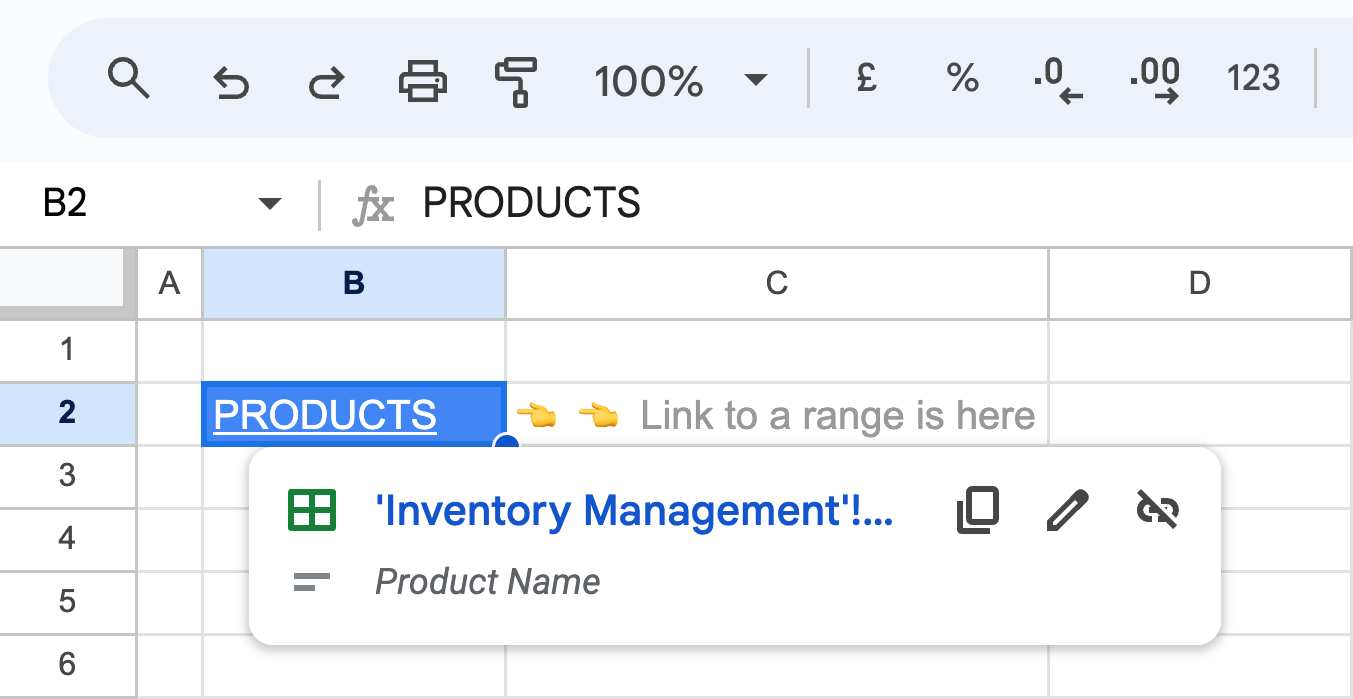
- Select the range, here C2:C12 on the Inventory Management tab, and name it “Products” under Data → Named ranges.
- In the cell that should hold the link, go to Insert → Link → Sheets and named ranges and choose Products.
Link two spreadsheets with IMPORTRANGE
Link two spreadsheets with IMPORTRANGE
References with a tab name only work inside one file. To bring in data from another spreadsheet, use IMPORTRANGE:
=IMPORTRANGE("spreadsheet_url", "range_string")
- spreadsheet_url: the URL of the source spreadsheet, in quotes.
- range_string: the tab name and range to import, in quotes, for example “Sales2024!B2:D100”.
The first time a spreadsheet imports from another one, the formula returns #REF! with the message that the sheets need to be connected. Click the cell and choose Allow access. You need at least view access to the source file.
Several imports can be stacked with curly braces and a semicolon. This puts two tabs of another spreadsheet under each other:
={IMPORTRANGE("https://docs.google.com/spreadsheets/d/16puodzCJMaUJuTjoYa-nDZ38N3sIWYMlt-OKznrkvGs/edit", "Sales2024!B2:D100");
IMPORTRANGE("https://docs.google.com/spreadsheets/d/16puodzCJMaUJuTjoYa-nDZ38N3sIWYMlt-OKznrkvGs/edit", "AnnualSales!B2:D100")}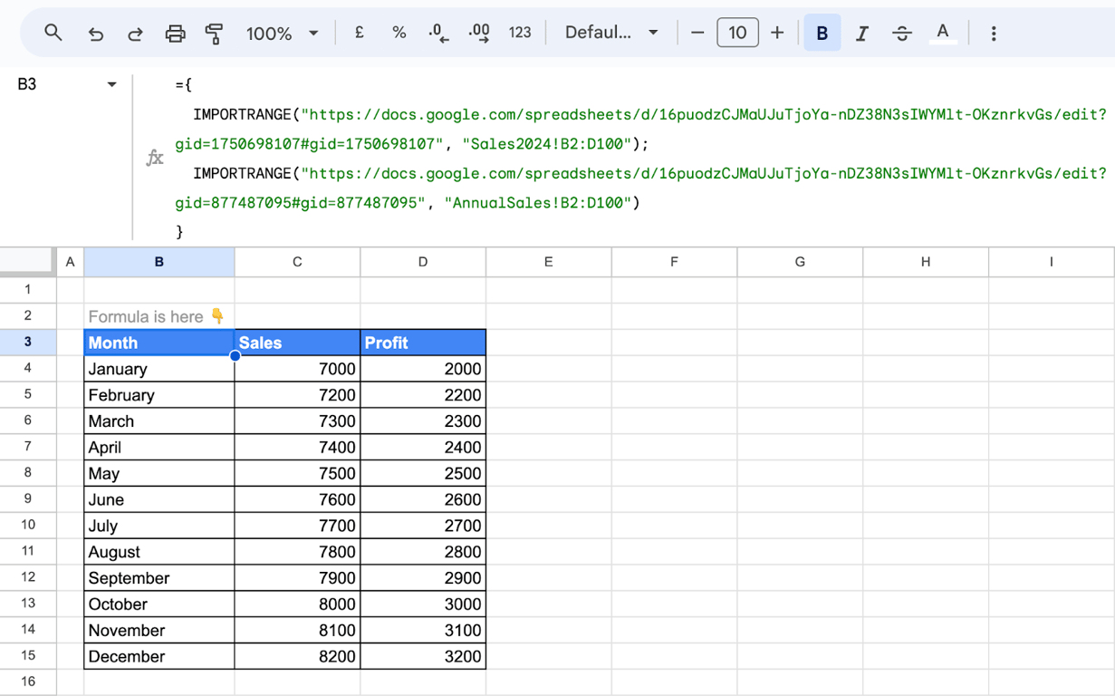

Problems when linking sheets, and how to fix them
Problems when linking sheets, and how to fix them
The import asks for access
❌ Error: IMPORTRANGE returns #REF!, or collaborators see errors where you see data.
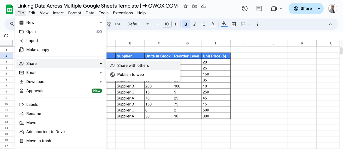
✅ Solution: Click the cell and allow access. Then check the sharing settings of the source file with the Share button: everyone who needs the linked data should have at least view access to the source.
Quotes are missing
❌ Error: The formula is rejected because the URL or the range is not in quotes.
=IMPORTRANGE(https://docs.google.com/spreadsheets/d/16puodzCJMaUJuTjoYa-nDZ38N3sIWYMlt-OKznrkvGs/edit, AnnualSales!A1:B10)
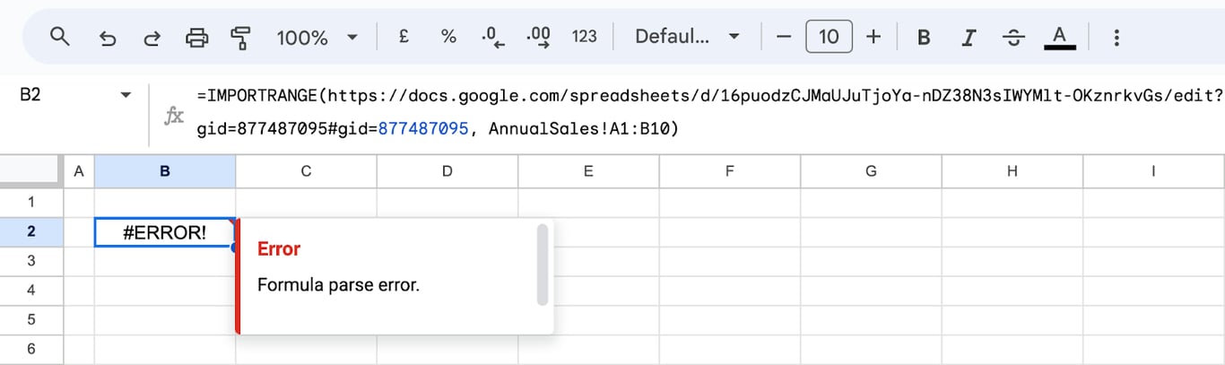
✅ Solution: Put both arguments of IMPORTRANGE in double quotes. In references inside the same file, put the tab name in single quotes when it contains a space.
The tab or the range does not exist
❌ Error: The formula returns #REF! because the tab named in it was renamed or deleted, or the range string is not valid.
=IMPORTRANGE("https://docs.google.com/spreadsheets/d/1ND3202nplI_2hFcgb-s4OUyDKkYGDQDGZ_rmEDgsxDg/edit", "DataSheet1!1:1")
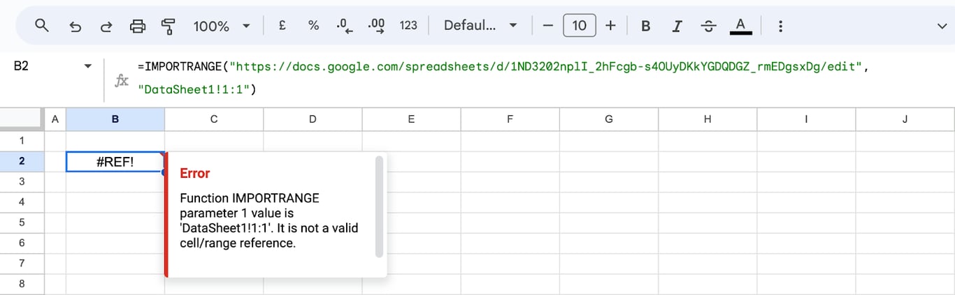
✅ Solution: Check the tab name and the range in the formula against the source. Direct references such as ‘Sales Orders’!A1 follow a renamed tab automatically. The text inside IMPORTRANGE and INDIRECT does not, and has to be corrected by hand.
Circular dependency
❌ Error: A formula refers to its own cell, directly or through other cells, and Google Sheets reports “Circular dependency detected”.
=SUM(A1:A10) + B1
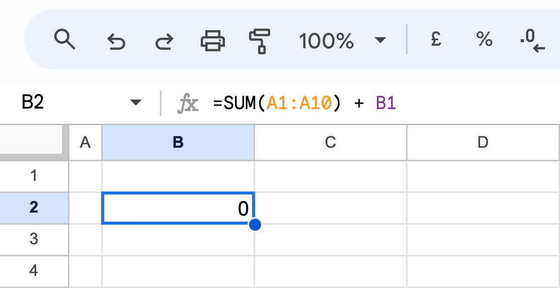
✅ Solution: Move the formula out of the range it refers to, or split the calculation across a helper cell so that no cell depends on itself.
The spreadsheet gets slow
❌ Error: A file with many cross-tab formulas and imports becomes slow to open and recalculate.
✅ Solution: Reference only the range you need instead of whole columns, delete unused rows and columns, and replace chains of IMPORTRANGE between many files with one source. A spreadsheet can hold up to 10 million cells; performance drops long before that.
Related Google Sheets functions
Related Google Sheets functions
Functions that are often used when linking data, each with its own guide:
- XLOOKUP: A more flexible lookup that can return values from any direction.
- IMPORTXML, IMPORTHTML and IMPORTFEED: Import data from web pages and feeds.
- UNIQUE: Returns the distinct values of a range.
- Pivot tables: Summarize data from a range by categories.
- MATCH: Returns the relative position of an item in a range.
- ARRAYFORMULA: Applies a formula to a whole column or range at once.
- IF: Returns one value when a condition is true and another when it is false.
- QUERY vs VLOOKUP: Compares the two functions and shows when each is the better choice.
- Currency conversion with GOOGLEFINANCE: Pulls current and historical exchange rates to convert amounts between currencies.
When the source is not a spreadsheet at all
When the source is not a spreadsheet at all
Everything above links one sheet to another sheet. That works until the data everyone depends on lives somewhere else: in a data warehouse, an ad platform or a CRM. Then the chain usually starts with someone exporting a file and pasting it into a “raw data” tab, and every IMPORTRANGE downstream faithfully copies whatever was pasted, however old it is.
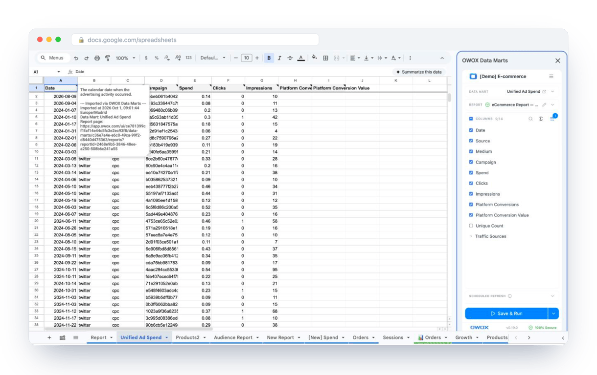
The OWOX Data Marts extension for Google Sheets replaces that first, manual link. A data analyst publishes a data mart (a table or an SQL query in your data warehouse) and makes it available for reports. You open the extension from the Extensions menu of the spreadsheet, pick the data mart, tick the columns you want and run it. The rows land in a tab, and your references, lookups and imports work on top of them.
What changes for the person who maintains the sheet:
- Refresh replaces re-export. Refresh current report re-runs the same pull, and a scheduled refresh keeps the tab current without anyone touching it.
- The source is written on the sheet. The header cell of an imported tab carries a note with the data mart it came from, the time of the import and a link to the report.
- No SQL and no warehouse access needed. The analyst decides which data marts and columns are available. You choose from that list.
The extension does not write or change the analyst’s SQL, and it does not replace the techniques in this guide: tabs still reference each other the same way. It makes the first tab in the chain trustworthy. When that tab needs columns from several warehouse tables, see joined Data Marts in Google Sheets. The extension comes with the OWOX Cloud plans of OWOX Data Marts; spreadsheet reporting describes both ways data reaches a sheet.
Turn your data into decisions.
Governed data marts give you the clean foundation ML needs to actually work.
- No AI hallucinations
- Analyst-governed definitions
- Every number traces to SQL
Frequently Asked Questions
What best practices should I follow while linking data across sheets?
When linking data across sheets in Google Sheets, follow these best practices to ensure data integrity and efficiency. Use named ranges for explicit and manageable references, employ array formulas for dynamic calculations, and consistently update cell references after sheet modifications. Leverage functions like IMPORTRANGE and QUERY to streamline data integration and real-time synchronization. Document any changes to maintain transparency and consistency across all linked data sources.
How can I use the QUERY function to import conditional data?
To import specific data based on conditions, use the QUERY function like this:=QUERY(IMPORTRANGE("spreadsheet_url", "range"), "SELECT columns WHERE condition")Here's a breakdown of the elements used in the formula:IMPORTRANGE: This function pulls data from another Google Sheet.spreadsheet_url: The web link to the Google Sheet you want to pull data from.range: The specific range of cells you want to import (e.g., "Sheet1!A1").QUERY: This function filters and organizes the imported data.SELECT columns: Specifies which columns to include in the results.WHERE condition: Sets the condition to filter the data (e.g., "WHERE D > 1000").
What should I do if I encounter REF errors due to invalid references?
If you encounter #REF errors in Google Sheets due to invalid references, verify that the referenced cells or ranges exist and have not been deleted or moved. Update or correct the affected formulas to point to valid references. Ensure that any referenced sheets are correctly named and accessible.Regularly auditing your sheets for #REF errors helps maintain data accuracy and prevents disruptions in data analysis workflows. Properly handling these errors is crucial for ensuring reliable and consistent data operations.
How can I import data using the IMPORTRANGE function from another sheet?
To import data from another sheet in Google Sheets, use the IMPORTRANGE function. The syntax is =IMPORTRANGE(spreadsheet_url, range_string), where spreadsheet_url is the link to the source sheet, and range_string specifies the data range.For example, =IMPORTRANGE will import the specified range. This function allows real-time data integration across sheets.
What are the benefits of linking data across multiple Google Sheets?
Linking data across multiple Google Sheets provides a lot of advantages, such as enhanced data consistency and accuracy. It allows for integrating disparate data sources, creating a centralized repository for comprehensive data analysis. This approach supports real-time updates, ensuring that any changes in source sheets are reflected across all linked documents. It also improves collaborative workflows by enabling different teams to access and update shared data seamlessly, optimizing operational efficiency.
How do I link data within the same Google Sheets document?
Use a reference with the tab name: ='Sheet2'!A1 shows cell A1 of the tab Sheet2, and ='Sheet2'!A1:C10 shows a range. The single quotes are needed when the tab name contains a space. You can also type =, click the other tab, click the cell and press Enter.