Cohort retention analysis in SQL: four choices that change the number
Any tutorial will give you the cohort retention query. What it will not tell you is how far the result moves with four choices you make on the way: which orders count, calendar months or rolling windows, exact month or any later month, and what to print for months that have not happened yet. This guide runs each choice in BigQuery on two datasets, prints every query with its result, gives a rule for an e-commerce orders table, and ends with a short note for the person who asked for the report.

“Can you send me cohort retention by month?” The query for that is about twenty lines, and every tutorial has it. This article is about the part they skip: four choices inside those lines change the number you report, and nobody asking for the table knows you made them.
Each choice below was run in BigQuery on 11 October 2026, on two datasets, with the query and the result printed. If you are the person who asked for the report, the last section is for you.
The short answer
For an e-commerce orders table, start from these defaults and write them under the table:
| Choice | Default for an orders table | What it did to the number here |
|---|---|---|
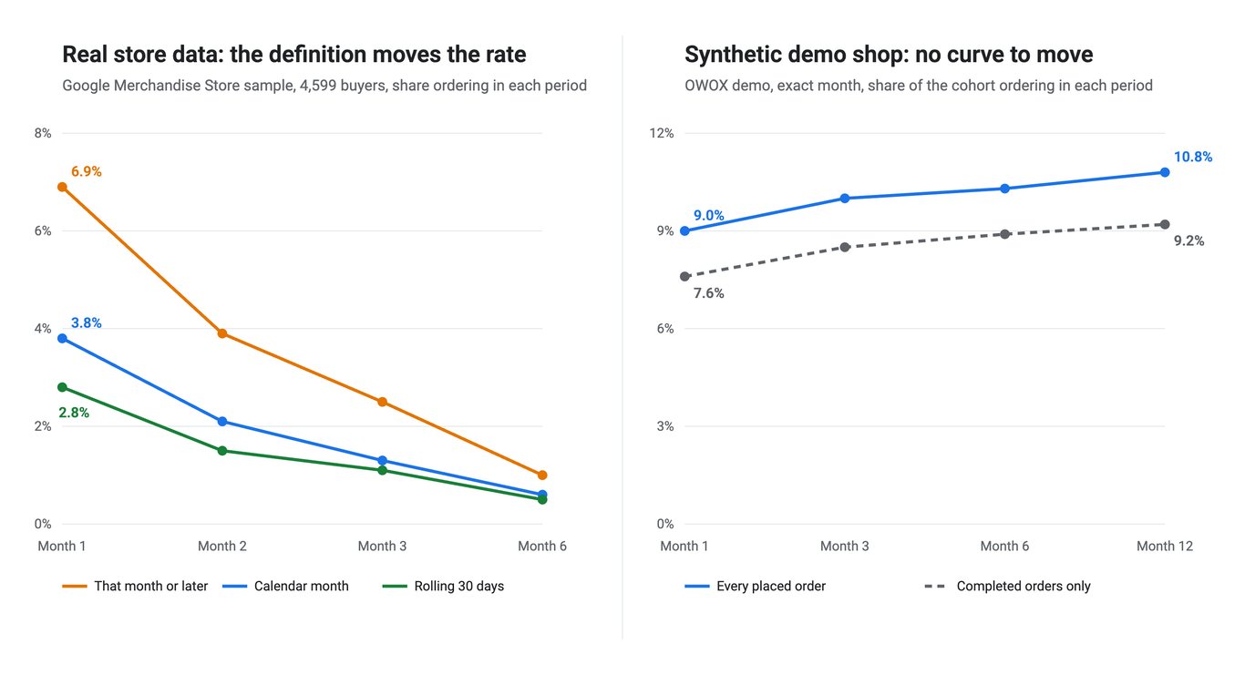
| Which orders count | Completed orders, for the first order and for the return | Month 1: 9.0% with every placed order, 7.6% with completed only |
| Calendar months or rolling 30-day windows | Rolling windows for a rate you will compare or act on; calendar months for a table people read next to monthly reports | Month 1 on real data: 3.8% calendar, 2.8% rolling |
| That month exactly, or that month or later | Exact month for the cohort table; “or later” only as a separate, labelled churn view | Month 1 on real data: 3.8% exact, 6.9% “or later” |
| Months that have not finished | Empty, never 0% | A July cohort at 0.7% in month 1 when its neighbours sit between 2.7% and 5.0% |
Two things decide the rest: whether the date you anchor the cohort on means what you think, and where your table starts. Both get a check query below.
The two datasets, and what each can show
The two datasets, and what each can show
No single public dataset shows all four choices, so this uses two. Read their limits before the numbers.
The OWOX demo shop (owox-demo.ecommerce, the storage behind the public [Demo] E-commerce project). It is synthetic, small and clean: 5,000 customers, 17,977 orders from 1 January 2024 to the day of the run, each with a status (15,272 Completed, 1,821 Cancelled, 884 Returned). It can show what order status does to retention, and what a wrong cohort date looks like. It cannot show a retention curve. Its orders are scattered across the months without relation to a customer’s first order, so about one customer in ten orders in any given month, whatever month they started in. You will see that flat line in the results. It is reported as it came out.
The Google Merchandise Store sample (bigquery-public-data.google_analytics_sample, which Google describes as “obfuscated Google Analytics 360 data from the Google Merchandise Store, a real ecommerce store” in its help article; the tables run from 1 August 2016 to 1 August 2017). It has real behaviour: 10,022 buyers, most of whom never return. Its limits: a “buyer” is a browser id (fullVisitorId), not a customer, so the same person on a phone and a laptop is two buyers and real retention is higher than these figures. An “order” is a session with at least one transaction. There is no order status. It is one store, nine years ago.
So the shape of the curve and the calendar effect come from the Google sample; the order-status effect comes from the demo. Neither is your data. Treat the sizes of the gaps as an illustration and the direction as the lesson.
OWOX Data Marts
See your first report built in real time. 15 minutes.
- Connect your data warehouse
- Pick your metrics
- Get a live Google Sheets report
In the time it takes to write a ticket. Then imagine never writing that ticket again.
Book a DemoWe'll use your actual use case
The base query, with every choice visible
The base query, with every choice visible
One query computes the definitions side by side, so the comparison is on the same rows. On the demo shop:
WITH orders AS (
  SELECT customer_id, order_date, status
  FROM `owox-demo.ecommerce.orders`
),
first_order AS (
  SELECT
    customer_id,
    MIN(order_date) AS first_placed,
    MIN(IF(status = 'Completed', order_date, NULL)) AS first_completed
  FROM orders
  GROUP BY customer_id
),
periods AS (SELECT k FROM UNNEST([1, 3, 6, 12]) AS k)
SELECT
  k AS period,
  COUNT(DISTINCT IF(f.first_placed BETWEEN '2024-01-01' AND '2025-08-31',
    f.customer_id, NULL)) AS cohort_placed,
  COUNT(DISTINCT IF(f.first_placed BETWEEN '2024-01-01' AND '2025-08-31'
    AND DATE_DIFF(DATE_TRUNC(o.order_date, MONTH),
                  DATE_TRUNC(f.first_placed, MONTH), MONTH) = k,
    f.customer_id, NULL)) AS placed_calendar,
  COUNT(DISTINCT IF(f.first_placed BETWEEN '2024-01-01' AND '2025-08-31'
    AND DIV(DATE_DIFF(o.order_date, f.first_placed, DAY), 30) = k,
    f.customer_id, NULL)) AS placed_rolling_30d,
  COUNT(DISTINCT IF(f.first_placed BETWEEN '2024-01-01' AND '2025-08-31'
    AND DATE_DIFF(DATE_TRUNC(o.order_date, MONTH),
                  DATE_TRUNC(f.first_placed, MONTH), MONTH) >= k,
    f.customer_id, NULL)) AS placed_unbounded,
  COUNT(DISTINCT IF(f.first_completed BETWEEN '2024-01-01' AND '2025-08-31',
    f.customer_id, NULL)) AS cohort_completed,
  COUNT(DISTINCT IF(f.first_completed BETWEEN '2024-01-01' AND '2025-08-31'
    AND o.status = 'Completed'
    AND DATE_DIFF(DATE_TRUNC(o.order_date, MONTH),
                  DATE_TRUNC(f.first_completed, MONTH), MONTH) = k,
    f.customer_id, NULL)) AS completed_calendar
FROM first_order AS f
CROSS JOIN periods
JOIN orders AS o USING (customer_id)
GROUP BY k
ORDER BY k
The cohort window stops at 31 August 2025 so that every customer in it has a finished month 12 under both the calendar and the rolling definition. The date arithmetic is DATE_TRUNC and DATE_DIFF, both covered in BigQuery date functions.
Result, demo shop, 11 October 2026 (customers, then share of the cohort):
| Period | Placed, calendar | Placed, rolling 30 days | Placed, that month or later | Completed, calendar |
|---|---|---|---|---|
| Cohort | 4,251 | 4,251 | 4,251 | 4,014 |
| 1 | 383 (9.0%) | 371 (8.7%) | 3,990 (93.9%) | 307 (7.6%) |
| 3 | 423 (10.0%) | 429 (10.1%) | 3,935 (92.6%) | 341 (8.5%) |
| 6 | 436 (10.3%) | 431 (10.1%) | 3,810 (89.6%) | 356 (8.9%) |
| 12 | 458 (10.8%) | 469 (11.0%) | 3,346 (78.7%) | 368 (9.2%) |
There is the flat line: 9.0% in month 1 and 10.8% in month 12. A real shop does not look like this.
The same query on the Google sample needs only a different orders CTE, no status columns, and its own cohort window (first purchase from 1 August to 31 December 2016, periods 1, 2, 3 and 6):
WITH orders AS (
  SELECT fullVisitorId AS buyer_id,
         PARSE_DATE('%Y%m%d', date) AS order_date
  FROM `bigquery-public-data.google_analytics_sample.ga_sessions_*`
  WHERE totals.transactions >= 1
),
first_order AS (
  SELECT buyer_id, MIN(order_date) AS first_placed
  FROM orders
  GROUP BY buyer_id
),
periods AS (SELECT k FROM UNNEST([1, 2, 3, 6]) AS k)
SELECT
  k AS period,
  COUNT(DISTINCT f.buyer_id) AS cohort,
  COUNT(DISTINCT IF(DATE_DIFF(DATE_TRUNC(o.order_date, MONTH),
    DATE_TRUNC(f.first_placed, MONTH), MONTH) = k,
    f.buyer_id, NULL)) AS placed_calendar,
  COUNT(DISTINCT IF(DIV(DATE_DIFF(o.order_date, f.first_placed, DAY), 30) = k,
    f.buyer_id, NULL)) AS placed_rolling_30d,
  COUNT(DISTINCT IF(DATE_DIFF(DATE_TRUNC(o.order_date, MONTH),
    DATE_TRUNC(f.first_placed, MONTH), MONTH) >= k,
    f.buyer_id, NULL)) AS placed_unbounded
FROM first_order AS f
CROSS JOIN periods
JOIN orders AS o USING (buyer_id)
WHERE f.first_placed BETWEEN '2016-08-01' AND '2016-12-31'
GROUP BY k
ORDER BY k
Result, Google Merchandise Store sample, 4,599 buyers, run on 11 October 2026:
| Period | Calendar month | Rolling 30 days | That month or later |
|---|---|---|---|
| 1 | 177 (3.8%) | 129 (2.8%) | 316 (6.9%) |
| 2 | 96 (2.1%) | 68 (1.5%) | 181 (3.9%) |
| 3 | 59 (1.3%) | 52 (1.1%) | 116 (2.5%) |
| 6 | 26 (0.6%) | 22 (0.5%) | 45 (1.0%) |
One note on naming: unbounded on its own is a reserved word in BigQuery, so a column called that fails with a syntax error. The first version of this query did.
Choice 1: which orders count
The rule: use completed orders for both ends, the order that puts a customer in a cohort and the order that counts as coming back. A cancelled order is not a customer you kept.
On the demo shop, counting every placed order gives 9.0% in month 1; counting completed orders only gives 7.6%. The gap holds at every period (10.8% against 9.2% in month 12): about a seventh of the rate. The cohort changes too, which is easy to miss. This check shows how:
WITH first_order AS (
  SELECT
    customer_id,
    MIN(order_date) AS first_placed,
    MIN(IF(status = 'Completed', order_date, NULL)) AS first_completed
  FROM `owox-demo.ecommerce.orders`
  GROUP BY customer_id
)
SELECT
  COUNT(*) AS customers,
  COUNTIF(f.customer_id IS NULL) AS never_ordered,
  COUNTIF(f.first_placed < c.registration_date) AS ordered_before_registering,
  COUNTIF(f.first_placed = c.registration_date) AS same_day,
  COUNTIF(f.first_placed > c.registration_date) AS ordered_after_registering,
  COUNTIF(f.customer_id IS NOT NULL
    AND f.first_completed IS NULL) AS no_completed_order,
  COUNTIF(DATE_TRUNC(f.first_completed, MONTH)
    > DATE_TRUNC(f.first_placed, MONTH)) AS cohort_month_moves
FROM `owox-demo.ecommerce.customers` AS c
LEFT JOIN first_order AS f USING (customer_id)| customers | never_ordered | ordered_before_registering | same_day | ordered_after_registering | no_completed_order | cohort_month_moves |
|---|---|---|---|---|---|---|
| 5,000 | 149 | 3,425 | 4 | 1,422 | 96 | 605 |
96 customers have orders and none completed, so they leave the table altogether. 605 move to a later cohort month, because their first completed order is in a later month than their first placed one. Mixing the two (cohort on any order, return on completed) is the version to avoid: it keeps people in the denominator who could never count in the numerator.
Where it gets harder: an order that is completed today and returned next week. Decide whether a return removes the order, and from which date, with whoever owns the revenue definition. The reconciliation of placed against completed order value covers that argument for money; retention inherits it.
The Google sample cannot test this choice. It has no status.
Choice 2: calendar months or rolling 30-day windows
Choice 2: calendar months or rolling 30-day windows
The rule: rolling windows from each customer’s own first order date when the rate will be compared or acted on; calendar months when the table has to sit next to monthly reports. Say which.
Calendar months put a customer who first buys on 30 January and again on 2 February into “month 1”, three days later. A customer who first buys on 1 January has to wait a month for the same label. Rolling windows give everyone the same clock: period 1 is days 30 to 59 after the first order.
On the Google sample the difference is large: 177 buyers (3.8%) in calendar month 1, 129 (2.8%) in the rolling window. Calendar months report 37% more month-1 retention from the same rows. The reason is in when people come back:
WITH orders AS (
  SELECT fullVisitorId AS buyer_id,
         PARSE_DATE('%Y%m%d', date) AS order_date
  FROM `bigquery-public-data.google_analytics_sample.ga_sessions_*`
  WHERE totals.transactions >= 1
),
first_order AS (
  SELECT buyer_id, MIN(order_date) AS first_placed
  FROM orders
  GROUP BY buyer_id
),
second_order AS (
  SELECT f.buyer_id, f.first_placed, MIN(o.order_date) AS second_placed
  FROM first_order AS f
  JOIN orders AS o USING (buyer_id)
  WHERE o.order_date > f.first_placed
  GROUP BY f.buyer_id, f.first_placed
)
SELECT
  COUNT(*) AS came_back,
  COUNTIF(DATE_DIFF(second_placed, first_placed, DAY) <= 29) AS within_29_days,
  COUNTIF(DATE_DIFF(second_placed, first_placed, DAY) <= 29
    AND DATE_TRUNC(second_placed, MONTH)
      = DATE_TRUNC(first_placed, MONTH)) AS same_calendar_month,
  COUNTIF(DATE_DIFF(second_placed, first_placed, DAY) <= 29
    AND DATE_TRUNC(second_placed, MONTH)
      > DATE_TRUNC(first_placed, MONTH)) AS next_calendar_month
FROM second_order
WHERE first_placed BETWEEN '2016-08-01' AND '2016-12-31'| came_back | within_29_days | same_calendar_month | next_calendar_month |
|---|---|---|---|
| 483 | 305 | 218 | 87 |
Of the 483 buyers who ever came back on a later day, 305 did it within 29 days. Calendar months split those quick returns by an accident of the date: 218 fell in the same calendar month and vanish into month 0, 87 crossed a month end and are counted as month-1 retention. A rolling window treats all 305 the same way.
On the demo shop the two definitions agree (9.0% and 8.7% in month 1). That is a null result, and it follows from how the data was made: orders that are spread evenly have no early returns to split. A synthetic table hides exactly the effect that moves a real report.
Choice 3: that month exactly, or that month or later
Choice 3: that month exactly, or that month or later
The rule: the cohort table uses the exact period. “That month or later” answers a different question, who has not churned yet, and belongs in its own view with its own label.
The two go by many names: classic, bounded or N-day retention for the exact period; unbounded or rolling retention for “or later”. On the Google sample, month 1 is 3.8% exact and 6.9% “or later”. Both are correct. They are not the same metric, and a tool that defaults to one will not match a query that uses the other.
The “or later” figure carries a trap. It can only fall, and part of the fall is the calendar running out. On the demo shop it reads 93.9% in month 1 and 78.7% in month 12. Nothing happened to those customers. There were simply fewer months left in which to see them again. On a fixed cohort window it is safe to read; on a live table, the newest cohorts always look worst.
The 93.9% itself is the demo’s randomness again: with orders scattered over 33 months, nearly everyone orders again at some point.
Choice 4: months that have not finished
Choice 4: months that have not finished
The rule: a cell whose period has not fully passed is empty. Not 0%, and not the partial figure.
The usual query has no notion of today. It prints whatever it finds, so the newest cohorts end in zeros and one partly counted month. This version adds the two things that are missing, a row for every cohort and period and a test of whether the period has ended:
WITH orders AS (
  SELECT fullVisitorId AS buyer_id,
         PARSE_DATE('%Y%m%d', date) AS order_date
  FROM `bigquery-public-data.google_analytics_sample.ga_sessions_*`
  WHERE totals.transactions >= 1
),
first_order AS (
  SELECT buyer_id, DATE_TRUNC(MIN(order_date), MONTH) AS cohort_month
  FROM orders
  GROUP BY buyer_id
),
cohort_size AS (
  SELECT cohort_month, COUNT(*) AS buyers
  FROM first_order
  GROUP BY cohort_month
),
activity AS (
  SELECT
    f.cohort_month,
    DATE_DIFF(DATE_TRUNC(o.order_date, MONTH), f.cohort_month, MONTH) AS period,
    COUNT(DISTINCT o.buyer_id) AS active
  FROM first_order AS f
  JOIN orders AS o USING (buyer_id)
  GROUP BY f.cohort_month, period
)
SELECT
  s.cohort_month,
  period,
  s.buyers,
  IFNULL(a.active, 0) AS active,
  ROUND(100 * IFNULL(a.active, 0) / s.buyers, 1) AS usual_pct,
  IF(LAST_DAY(DATE_ADD(s.cohort_month, INTERVAL period MONTH))
       <= DATE '2017-08-01',
     ROUND(100 * IFNULL(a.active, 0) / s.buyers, 1), NULL) AS ripe_pct
FROM cohort_size AS s
CROSS JOIN UNNEST(GENERATE_ARRAY(0, 6)) AS period
LEFT JOIN activity AS a
  ON a.cohort_month = s.cohort_month AND a.period = period
ORDER BY s.cohort_month, period
The date in the test is the last day the data covers. On a live table, use yesterday. Result for periods 1 to 3, all thirteen cohorts, with the cells the test blanks shown in brackets:
| Cohort | Buyers | Month 1 | Month 2 | Month 3 |
|---|---|---|---|---|
| 2016-08 | 1,046 | 46 (4.4%) | 21 (2.0%) | 13 (1.2%) |
| 2016-09 | 747 | 28 (3.7%) | 7 (0.9%) | 6 (0.8%) |
| 2016-10 | 769 | 40 (5.2%) | 27 (3.5%) | 17 (2.2%) |
| 2016-11 | 804 | 41 (5.1%) | 25 (3.1%) | 8 (1.0%) |
| 2016-12 | 1,233 | 22 (1.8%) | 16 (1.3%) | 15 (1.2%) |
| 2017-01 | 591 | 17 (2.9%) | 10 (1.7%) | 2 (0.3%) |
| 2017-02 | 606 | 26 (4.3%) | 17 (2.8%) | 12 (2.0%) |
| 2017-03 | 726 | 33 (4.5%) | 9 (1.2%) | 12 (1.7%) |
| 2017-04 | 796 | 40 (5.0%) | 11 (1.4%) | 3 (0.4%) |
| 2017-05 | 967 | 26 (2.7%) | 16 (1.7%) | [1 (0.1%)] |
| 2017-06 | 813 | 37 (4.6%) | [0 (0.0%)] | [0 (0.0%)] |
| 2017-07 | 890 | [6 (0.7%)] | [0 (0.0%)] | [0 (0.0%)] |
| 2017-08 | 34 | [0 (0.0%)] | [0 (0.0%)] | [0 (0.0%)] |
Look at July 2017: 0.7% in month 1, against 2.7% to 5.0% for the three cohorts before it. Nothing went wrong in July. The data ends on 1 August, so that cell holds one day of August. On a dashboard it reads as a collapse.
The same cells bend any average. Add up month 1 across all thirteen cohorts and you get 362 of 10,022 buyers, 3.6%. Leave out the two cohorts whose month 1 has not finished and it is 356 of 9,098, 3.9%. For month 3 the gap is wider: 89 of 10,022 (0.9%) against 88 of 7,318 (1.2%). Including unfinished months understated month-3 retention by a quarter.
The demo shop shows the same thing with today’s date (the same query with the demo orders CTE filtered to status = 'Completed' and 10 October 2026 as the last full day). Its November 2025 cohort prints 0.0% for month 12, a month that has not started, and its December 2025 cohort prints 2.7% for month 10, which is ten days of October 2026.
Two checks before you trust the cohort date
Two checks before you trust the cohort date
Does the date mean what you think?
A cohort is only as good as the date that defines it. “Registration date” sounds like the start of a customer. In the demo shop it is not: the check under choice 1 shows 3,425 of the 4,851 customers with an order placed their first order before their registration date. A cohort table built on that column would show customers “retained” in months before they existed.
In the demo this comes from how the data was generated. In a real shop the same pattern has ordinary causes: guest checkout, an account created at the second purchase, a migration that reset the field. Run the comparison once for whatever date you plan to anchor on. If a meaningful share of first orders precede it, anchor on the first order instead.
Where does the table start?
The first cohort in any table contains everyone whose earlier history is missing. They are counted as new, and they are not.
WITH first_order AS (
  SELECT customer_id, DATE_TRUNC(MIN(order_date), MONTH) AS month
  FROM `owox-demo.ecommerce.orders`
  GROUP BY customer_id
),
new_buyers AS (
  SELECT month, COUNT(*) AS first_order_customers
  FROM first_order
  GROUP BY month
),
buyers AS (
  SELECT DATE_TRUNC(order_date, MONTH) AS month,
         COUNT(DISTINCT customer_id) AS customers_ordering
  FROM `owox-demo.ecommerce.orders`
  GROUP BY month
),
registered AS (
  SELECT DATE_TRUNC(registration_date, MONTH) AS month,
         COUNT(*) AS registrations
  FROM `owox-demo.ecommerce.customers`
  GROUP BY month
)
SELECT month, first_order_customers, customers_ordering, registrations
FROM new_buyers
JOIN buyers USING (month)
JOIN registered USING (month)
WHERE month IN ('2024-01-01', '2025-01-01', '2026-01-01', '2026-09-01')
ORDER BY month| month | first_order_customers | customers_ordering | registrations |
|---|---|---|---|
| 2024-01 | 309 | 309 | 151 |
| 2025-01 | 130 | 414 | 152 |
| 2026-01 | 43 | 480 | 145 |
| 2026-09 | 16 | 579 | 135 |
In January 2024, the first month of the table, every one of the 309 customers who ordered is “new”. By September 2026 there are 16 new customers a month while 579 order and registrations have not moved. Read as acquisition, that is a business that stopped finding customers. It is a fixed pool of 5,000 being seen for the first time, most of them early.
Your table has a milder version of the same edge. If the orders table begins at a migration or a retention cut-off, drop the first cohorts or mark them, and never read their size as acquisition.
The line to print under every cohort table
The line to print under every cohort table
A cohort table without its definition invites the question “why doesn’t this match?”. Print the choices where the reader sees them:
Customers by month of first completed order. Retained = at least one completed order in that calendar month. Share of the original cohort. Months that have not ended are empty. Orders from 1 January 2024; the first three cohorts include customers with earlier history. Data to 10 October 2026.
Six short sentences. Each one answers a question that otherwise arrives as a message a week later. If the business uses the table to judge campaigns, add which cohorts are large enough to read: a cohort of 34 buyers moves three points when one of them returns.
For the definitions behind the metric itself, see customer retention rate; for cohort analysis without SQL, in Google Analytics and Google Sheets, see the introduction to cohort analysis.
What happens when someone asks an AI assistant instead
What happens when someone asks an AI assistant instead
The same choices get made when nobody writes SQL at all. To see how, the retention question was put to an AI assistant connected to the demo project through the MCP server of OWOX Data Marts, in three phrasings, on 11 October 2026.
How the test was run, so you can weigh it: the assistant was Claude, in a fresh session for each phrasing, given the question and nothing else, limited to the OWOX tools, at most seven tool calls and three data queries. It is one run per phrasing. The demo project has Data Marts for orders, customers and visitors. None of them defines retention, and that is the condition being tested.
| Asked | What the assistant did | What came back |
|---|---|---|
| “What is our customer retention rate?” | Looked for a retention metric in the Customers Data Mart and one report, found none, and stopped | No number. “I can’t give you a customer retention rate from the data I can reach, and I’d rather not hand you a made-up proxy.” It proposed a definition of its own: a repeat completed order within 12 months |
| “Of the customers who placed their first order in January 2025, how many came back and ordered again in the next month?” | Two queries on the Orders Data Mart: first order date per customer, then February orders for those customers | “9 of the 130 customers”, 6.9%, any order status, calendar February. It added the completed-only count unprompted: 7, about 5.4% |
| “Show me monthly cohort retention for customers acquired in the first half of 2025.” | Grouped customers by registration month, counted those with a completed order in each later month | A full table. Month 0 is 6.6% for the January cohort, not 100%, and it said why: these customers were ordering before they registered |
The middle answer can be checked against the SQL above: the January 2025 cohort is 130 customers in both, and 9 of them ordered in February in both. The two queries it sent, as sent (the list of 130 ids is shortened here):
{"data_mart_id": "d565c4cb-5f68-480e-917d-c1709b59ae02",
 "fields": ["customer_id", "order_date"],
 "aggregations": [{"field": "order_date", "function": "MIN"}],
 "filters": [
   {"field": "order_date", "operator": "lte", "value": "2025-01-31"},
   {"field": "customer_id", "operator": "is_not_blank"}],
 "sort": [{"field": "order_date", "direction": "desc"}],
"limit": 1000}{"data_mart_id": "d565c4cb-5f68-480e-917d-c1709b59ae02",
"fields": ["customer_id", "order_date", "orders_total", "completed_orders"],
"aggregations": [{"field": "order_date", "function": "MIN"}],
"filters": [
{"field": "order_date", "operator": "between",
"value": {"from": "2025-02-01", "to": "2025-02-28"}},
{"field": "customer_id", "operator": "in", "value": [2393, 471, 4229]}],
"sort": [{"field": "order_date", "direction": "asc"}],
"limit": 1000}The first returned 1,000 rows and was cut off at the row limit; the assistant sorted by date so the January customers came first, counted 130 of them by hand and said so. The second returned 9 rows with totals of 9 orders and 7 completed orders, computed by the Data Mart’s own orders_total and completed_orders fields.
What the trace shows:
- Three phrasings, three definitions. No number, first-order cohort with any status, registration cohort with completed orders. Each was a reasonable reading of the words. None was wrong on its own terms, and they cannot be compared with each other.
- Where a definition existed, it was used. The completed-order count came from a field the Data Mart defines, not from the assistant’s own arithmetic.
- Where none existed, the assistant chose, or declined. It disclosed every choice, which is the best case. It still made them for you.
- The registration trap is real. One phrasing walked straight into the cohort date that 3,425 customers contradict. The assistant noticed and said so; a table pasted into a slide would not carry that warning.
The consequence for the analyst is the same as for a dashboard. If the cohort query above lives in a Data Mart, with the definition line as its description, then the question is answered from your SQL instead of being rebuilt from raw orders under a row limit. That Data Mart was not built for this article, so there is no trace of it to show. Two limits apply either way: the rows an assistant reads are sent to the AI provider, and a written definition does not make every answer identical. What it gives is the same definitions behind every answer, and a calculation you can open.
In OWOX Data Marts, a Data Mart is defined with SQL, a table or a view and carries a description and field descriptions (core concepts). The same Data Mart can be delivered to Google Sheets on a schedule with a report run trigger (docs), and read by assistants through the MCP server (docs). Whether an AI answer deserves trust at all is a separate question, worked through in can you trust AI with business numbers.
For the person who asked for the report
For the person who asked for the report
If you asked your analyst for “cohort retention” and got questions back instead of a table, they were the right questions. Here is the short version.
Retention is not one number. It is the share of customers who came back, and “came back” has to be spelled out. On one real shop’s data, the same customers gave 3.8% or 2.8% for the first month, depending only on whether a month means the calendar month or thirty days from each customer’s first order. Counting every order, or only the ones that were not cancelled, moved another dataset from 9.0% to 7.6%.
Three things only you can decide:
- Which orders count. Cancelled and returned orders: in or out? Out is the safer default. If finance already has a rule for what counts as a sale, use theirs.
- What you will use the table for. To sit beside monthly reports, calendar months are fine. To judge whether one month’s customers were better than another’s, ask for thirty-day windows.
- Who signs off the definition. One sentence under the table, agreed once, saves the argument every time the number is quoted.
Two things to stop doing:
- Do not read the newest rows. The most recent months are still filling up, and a good table leaves them blank. A low figure for last month’s customers usually means the month is not over.
- Do not compare this table with the retention figure in another tool until you know both use the same definition. They usually do not.
Once those three decisions are written down, the table will mean the same thing next quarter as it does today.
Turn your data into decisions.
Governed data marts give you the clean foundation ML needs to actually work.
- No AI hallucinations
- Analyst-governed definitions
- Every number traces to SQL
Frequently Asked Questions
How do you calculate cohort retention in SQL?
Give each customer a cohort from their first order (`MIN(order_date)`, cut to the month with `DATE_TRUNC`), measure how far every later order is from that date with `DATE_DIFF`, count distinct customers per cohort and period, and divide by the size of the cohort. Both functions are in BigQuery's date function reference. The query is short; the result depends on four choices you make inside it: which orders count, calendar months or rolling windows, the exact period or any later one, and what to print for periods that have not ended.
Should cohort retention use calendar months or 30-day windows?
Use rolling 30-day windows from each customer's first order when you will compare cohorts or act on the rate, and calendar months when the table has to sit next to monthly reports. They can differ a lot. On Google's public Google Merchandise Store sample, the same 4,599 buyers gave 3.8% retention in calendar month 1 and 2.8% in the rolling window (our run in BigQuery, 11 October 2026), because calendar months count a return a few days later as "month 1" whenever a month end falls in between.
What is the difference between classic and unbounded retention?
Classic (also called bounded or N-day) retention counts customers who were active in exactly that period. Unbounded (also called rolling) retention counts customers active in that period or any later one, so it is the share who have not churned yet. On Google's public Google Merchandise Store sample, month 1 was 3.8% classic and 6.9% unbounded for the same buyers (our run in BigQuery, 11 October 2026). Unbounded retention always makes the newest cohorts look worst, because they have had less time to return.
Why does the newest cohort in a retention table look worse?
Usually because its latest period has not finished. The standard query has no notion of today, so it prints a partly counted month as if it were complete, and months that have not started as 0%. In Google's public Google Merchandise Store sample, which ends on 1 August 2017, the July 2017 cohort shows 0.7% in month 1 while the three cohorts before it show 2.7% to 5.0% (our run in BigQuery, 11 October 2026): that cell holds one day of August. Leave a cell empty until its period has fully passed.
Should cancelled and returned orders count in cohort retention?
For most e-commerce reporting, no: use completed orders both for the first order that defines the cohort and for the order that counts as a return. On the synthetic OWOX demo shop, month-1 retention was 9.0% with every placed order and 7.6% with completed orders only, 96 of 4,851 ordering customers dropped out because none of their orders completed, and 605 moved to a later cohort month (our run in BigQuery, 11 October 2026). If finance already has a rule for what counts as a sale, use that rule.