How to Use Data Validation in Google Sheets for Clean Data

Keeping data clean in Google Sheets can be tricky, especially when many people are entering information. One small mistake can throw off calculations, reports, or inventory tracking. 

That’s where data validation comes in. It helps control what kind of data can be entered in each cell. It’s an easy way to reduce errors and keep your spreadsheet organized. 

This guide will walk you through how to use data validation in Google Sheets. You’ll learn basic steps, advanced options, and how to fix common issues. Whether you manage sales data or team reports, these tips can help you keep everything accurate and reliable.

What Is Data Validation in Google Sheets?  

Data validation in Google Sheets is a feature that lets you set rules for what kind of data can be entered in specific cells. You can limit input to things like numbers within a certain range, valid dates, or text from a dropdown list. If someone enters data that doesn't match the rule, they’ll get a warning or the input may be rejected.

This is helpful when dealing with important data, like sales figures or reports. For example, you can allow only values between 0 and 1,5000 to avoid incorrect entries. It also helps catch common mistakes and keeps your spreadsheet clean and accurate.

Importance of Data Validation in Google Sheets 

Here’s why data validation is important when working in Google Sheets. These points highlight how it helps you manage data more effectively and avoid common issues.

• Prevents Errors: It stops users from entering incorrect, incomplete, or mismatched data. This helps avoid small mistakes that can affect calculations or reports.
• Ensures Consistency: Validation keeps formats, values, and data types the same across your sheet. This makes your data cleaner and easier to work with.
• Saves Time: By catching mistakes early, you won’t need to spend hours reviewing or fixing errors later.
• Improves Data Quality: It helps you maintain accurate and meaningful data, which leads to better insights and decisions.
• Supports Teamwork: When working with others, validation keeps entries consistent, reducing confusion and making collaboration more reliable.

How to Use Data Validation in Google Sheets for Clean Data Ready-to-use Template!

This downloadable file contains all the examples from the article, allowing you to practice and implement How to Use Data Validation in Google Sheets for Clean Data in your own projects. Download, explore, and start mastering data validation in Google Sheets with ease!

Get your free template now

Steps for Setting Up Basic Data Validation

Setting up basic data validation helps keep your data accurate from the start. Here’s how you can apply a simple rule step by step: 

Example:

Suppose you’re working with a sales team dataset and want to make sure the Lead Score column only accepts values between 1 and 10.

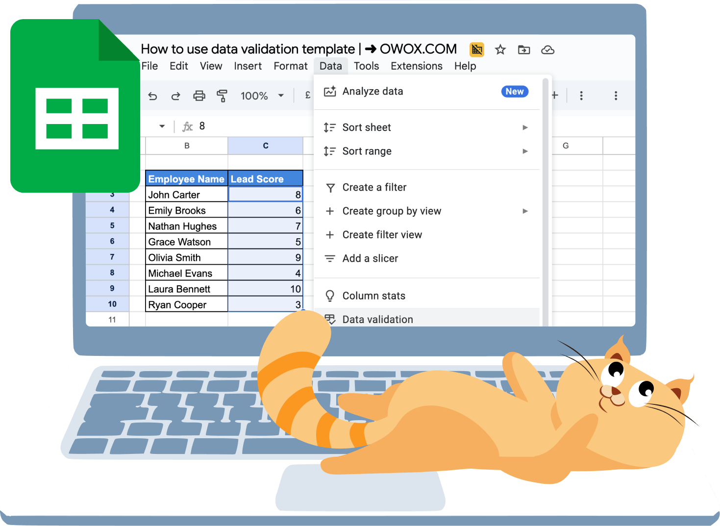
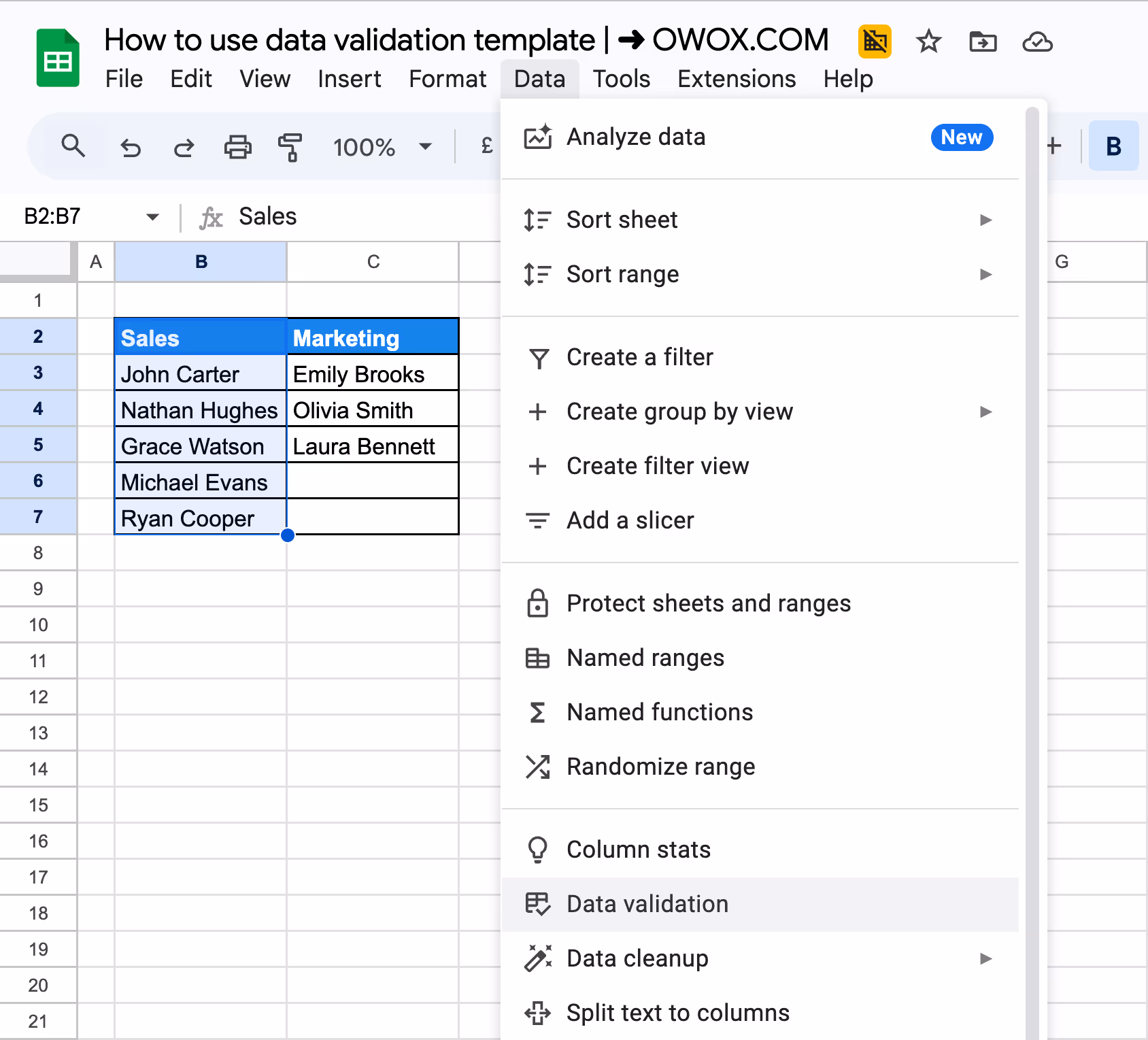
Step 1: Right-click the column header where you want to apply the rule and choose Data validation. You can also go to the top menu and click Data > Data validation.

Step 2: In the sidebar that appears, click + Add rule to start setting up your validation.

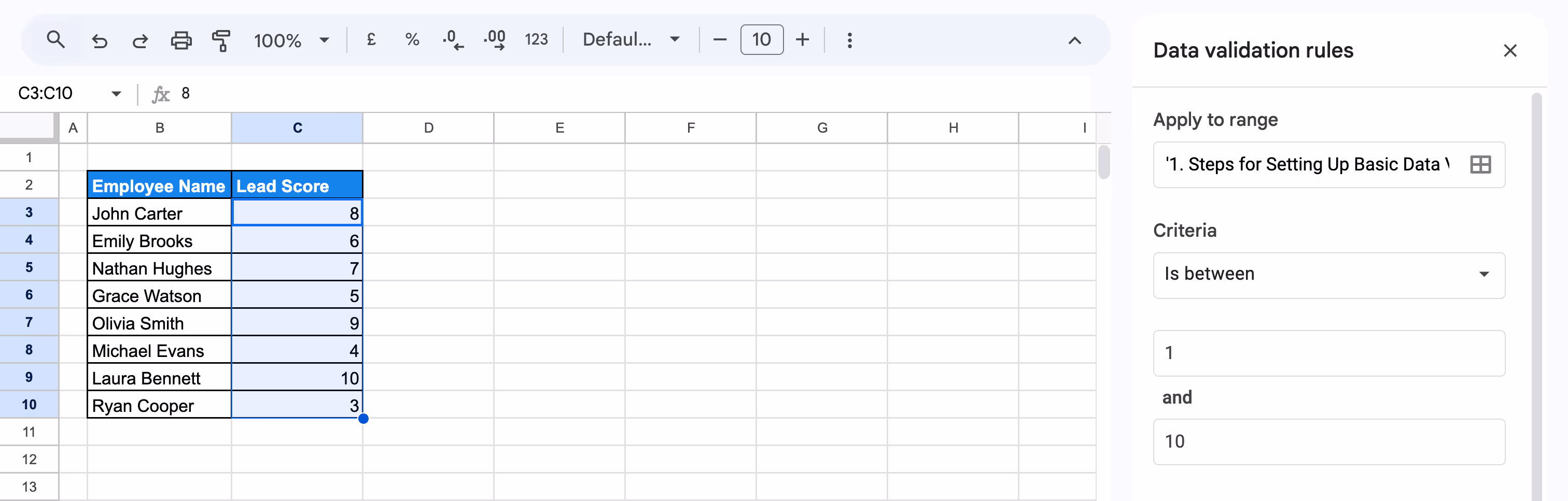
Step 3: Check the Apply to range box to confirm the selected cells are correct. This is where your rule will be applied.

Step 4: Under Criteria, choose a condition such as Is between, and enter limits like 1 and 10. 

Step 5: Choose how invalid entries are handled, either show a warning or block the input completely with Reject input, and click on Done to apply the rule.

Data validation rule applied to the Lead Score column, restricting values to between 1 and 10. When an invalid entry is made, a warning message appears to guide the user.

Basic Usage of Data Validation Rules in Google Sheets 

Basic data validation helps control what users can enter in your spreadsheet. You can set rules for numbers, text, dates, dropdown lists, and more to keep your data clean and consistent.

Creating a Drop-Down List with Data Validation

Adding a dropdown list with data validation is a simple way to limit input to specific values, reducing mistakes and saving time. It ensures your data stays clean and consistent. 

Example:

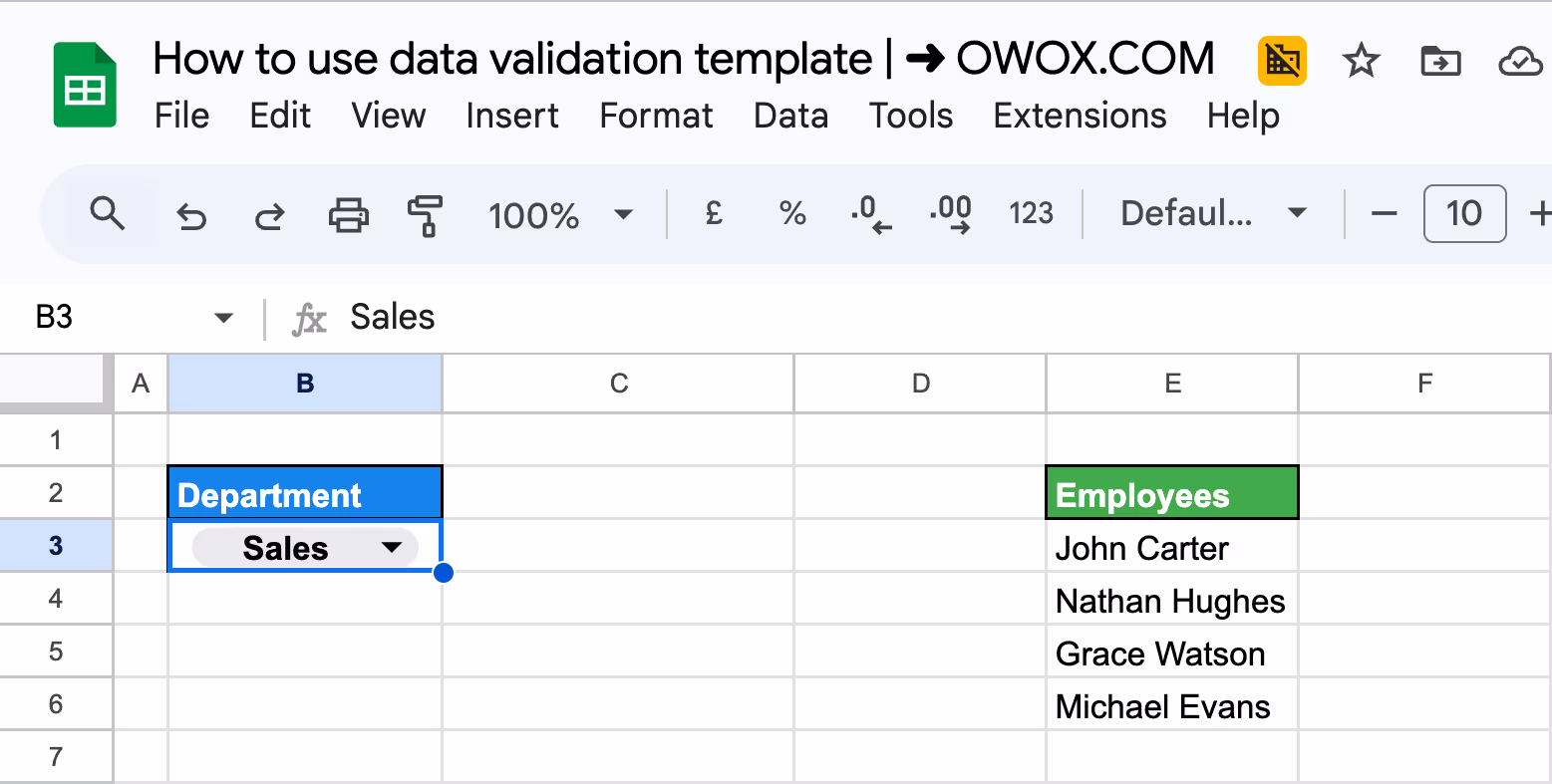
Suppose you're working with a team dataset and want to ensure only "Sales" or "Marketing" is entered under the Department column.

Steps to create the dropdown list:

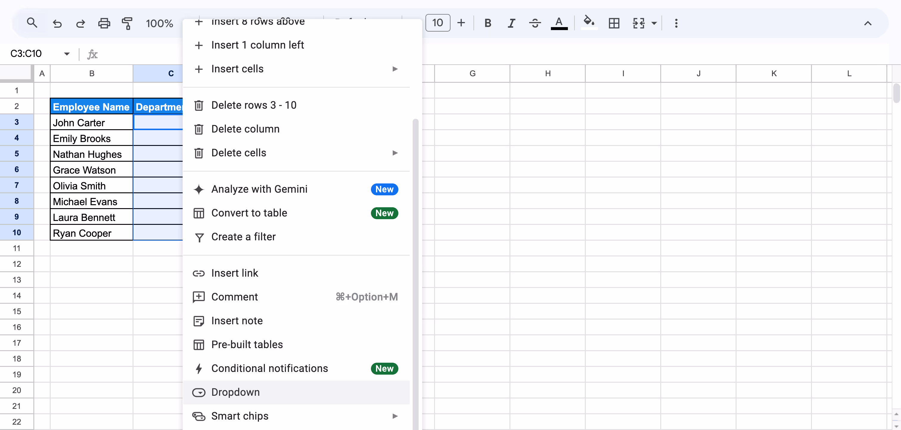
Step 1: Highlight cells C3 to C10 in the Department column. Click Data > Data validation or right-click and choose Dropdown.

Step 2: In the setup panel, choose Drop-down as criteria and enter the allowed values: Sales and Marketing. 

Step 3: Click Done, then test the dropdown to confirm it works. 

A dropdown list applied to the Department column, allowing only “Sales” or “Marketing” as valid inputs.

Setting Up Number Validation

When working with numerical data, it’s important to make sure the values entered fall within a logical range. Number validation helps prevent errors that can affect calculations and reporting.

Example:

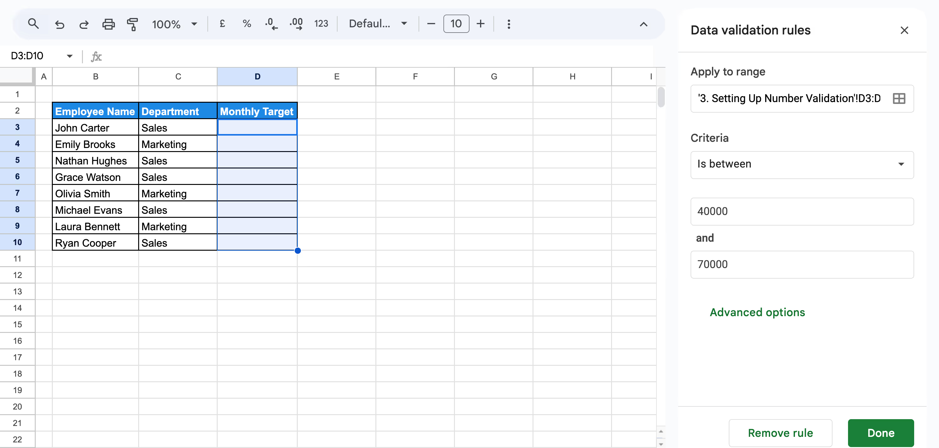
Suppose you want to ensure the Monthly Target column only accepts values between $40,000 and $70,000.

Steps to set up a number validation:

Step 1: Select the cells in the Monthly Target column that contain or will contain numeric data, and click on Data > Data validation from the top menu. 

Step 2: In the sidebar, set Criteria to is between and enter 40000 as the minimum and 70000 as the maximum value. Click Done to finish and activate the validation rule.

Step 3: Test the rule by entering a value like, 30000 to see if the error message appears for numbers outside the allowed range.

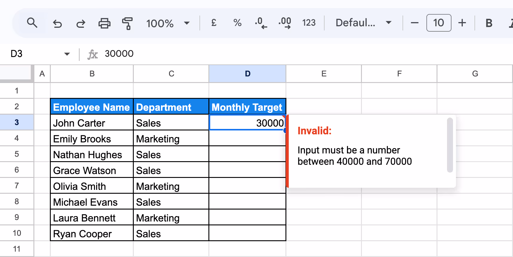
This ensures only valid monthly target values are entered, keeping your data accurate and within the set limits.

Applying Text Validation

Text validation helps ensure users enter information in a consistent format, especially in fields like email addresses, where accuracy matters.

Example:

Suppose you want to make sure all entries in the Email column are valid email addresses.

Steps to apply text validation:

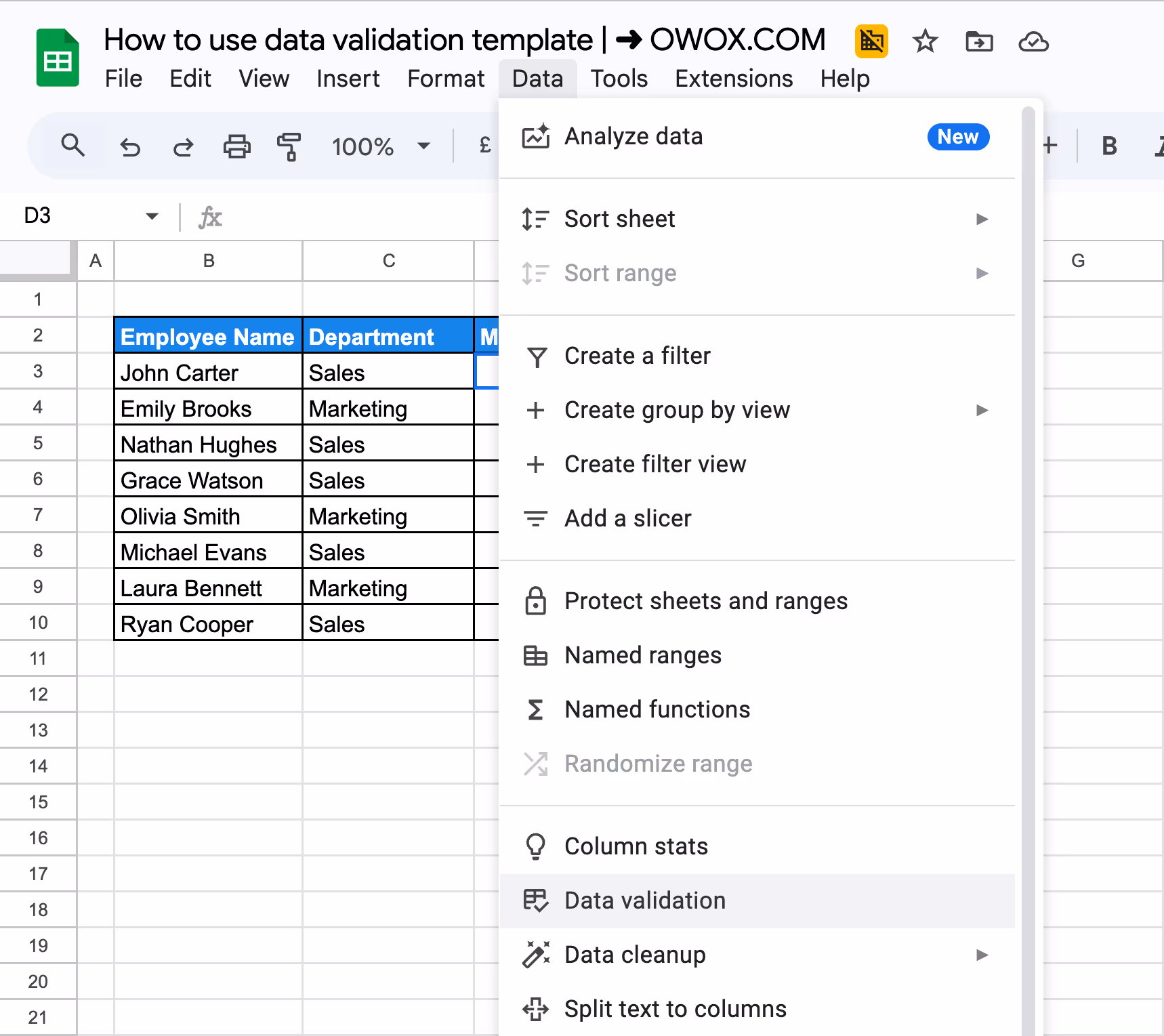
Step 1: Select the cells in the Email column where email addresses will be entered. Click on Data > Data validation from the top menu to open the sidebar.

Step 2: Under Criteria, choose the “Text is valid email” option from the dropdown options. 

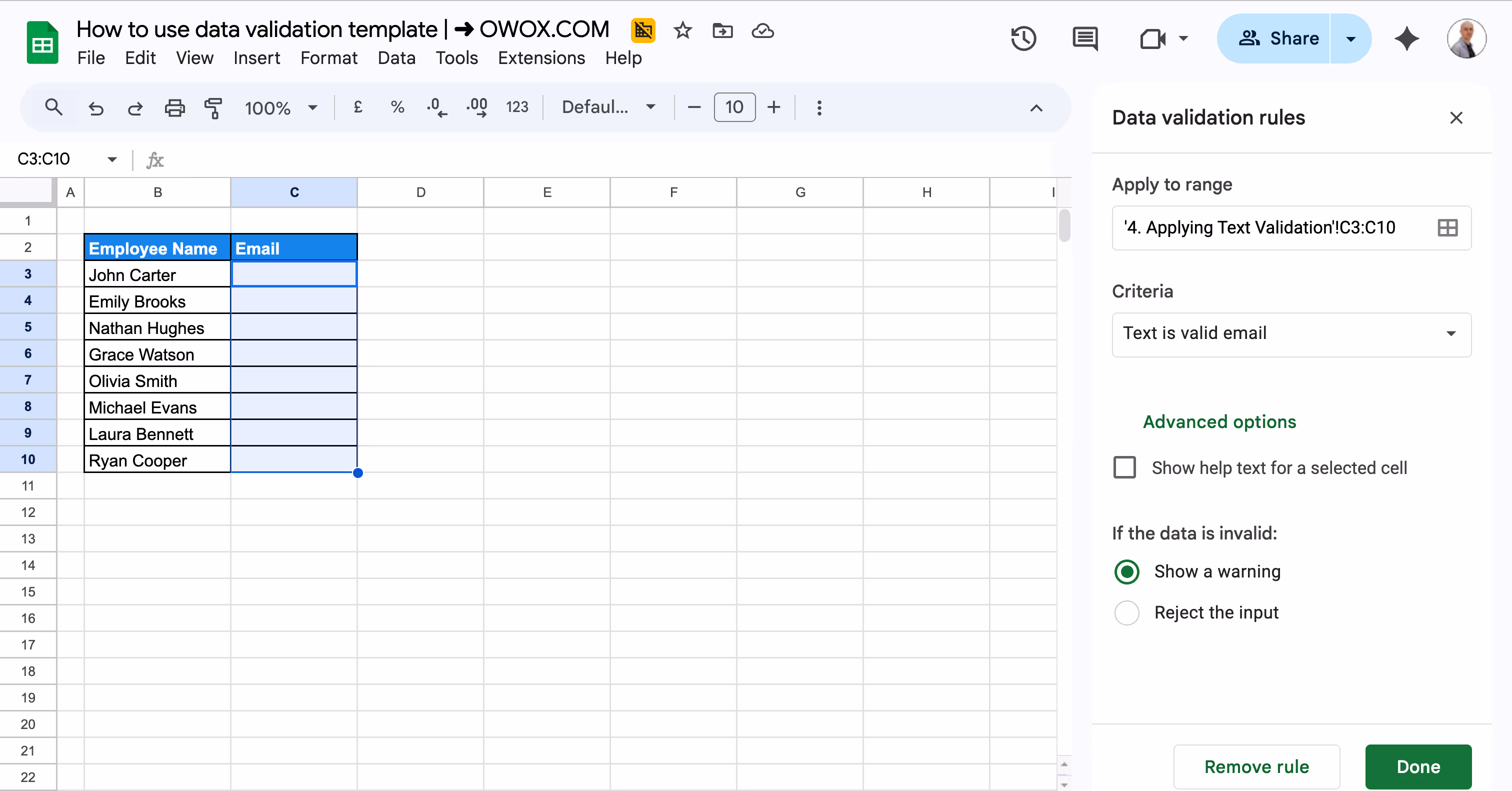
Under the Advanced option, add a help text like “Please enter a valid email address” to make sure any wrong input can't be given; the help text can be anything you like. Make sure you select “Reject the output” under “If the data is invalid”.

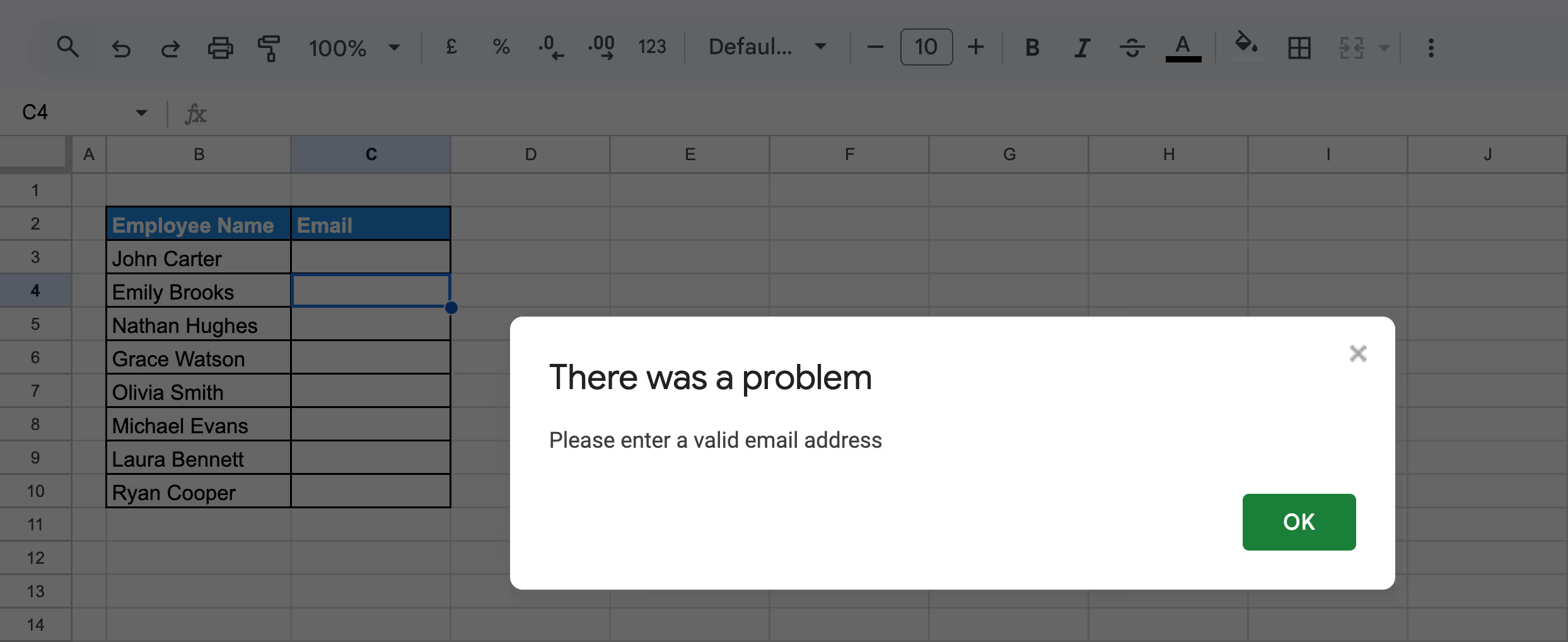
Test it by typing an incorrect email to see if the rule works. If you don't select the Reject output option, users will see the following error.

This example validates the email format correctly using the built-in "Text is valid email" rule in Google Sheets.

Setting Up Date Validation

Date validation ensures that only proper date formats are entered into your spreadsheet. This helps prevent issues caused by typos, text entries, or incomplete dates.

Example:

Suppose you want to make sure all entries in the Join Date column are valid dates, not random text or incorrectly typed values.

Steps to apply date validation:

Step 1: Select the cells in the Join Date column where team members' joining dates are going to be entered and click Data > Data validation to open the rule panel.

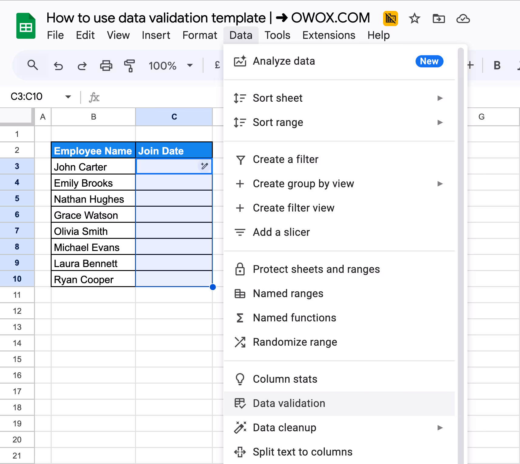
Step 2: Under Criteria, choose “Is valid date” from the dropdown options. Click Done to save and apply your rule to the selected cells. 

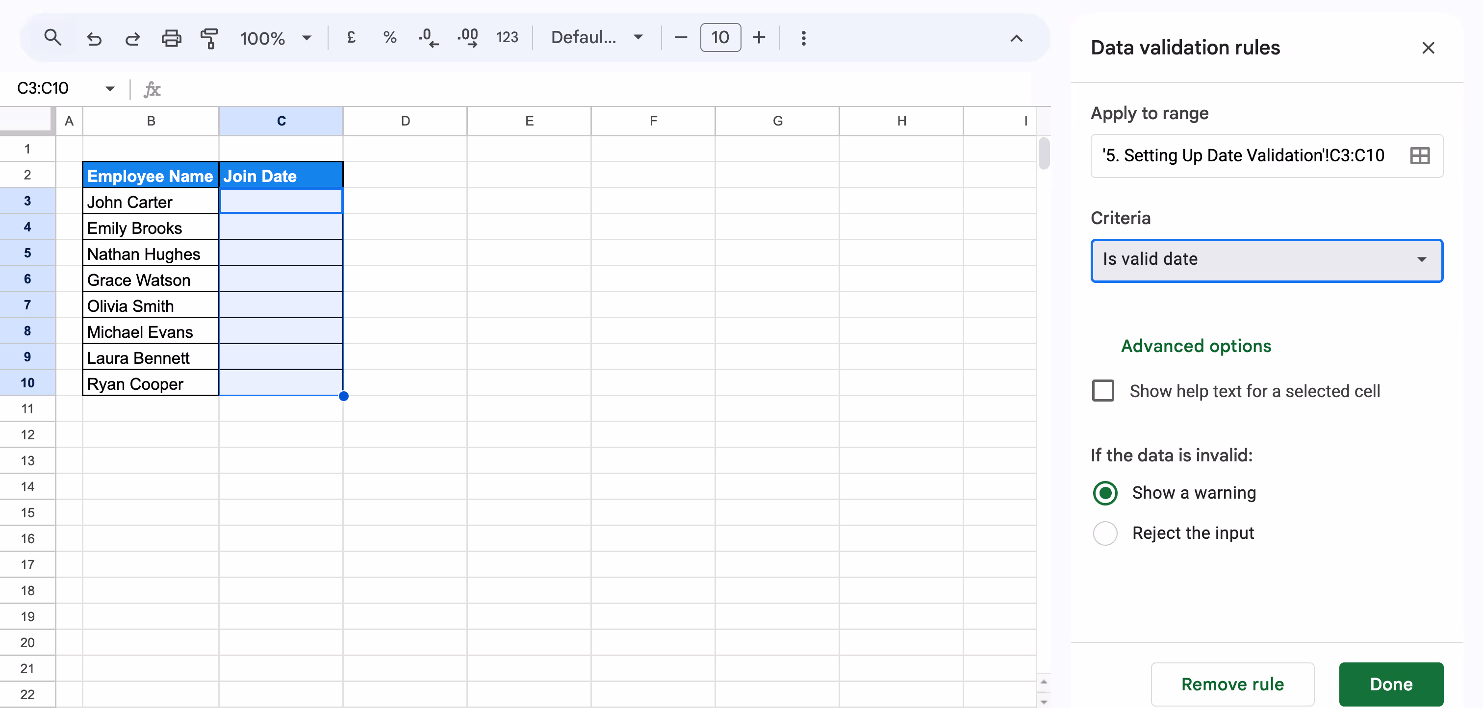
Test it by entering something like "Next Monday" or "Joined last year" to see if it's blocked. 

A calendar will appear when you click the cell, allowing you to select a date in the correct format.

This ensures that only valid calendar dates are accepted, keeping your date-related data clean and consistent.

Using a Checkbox for Binary Validation

Checkbox validation restricts input to two clear options – checked or unchecked. It's useful for tracking simple yes/no data, like task completion or employee status.

Example:

Suppose you want to track if an employee is active using the Active column in your dataset.

Steps to apply checkbox validation:

Step 1: Select the cells in the Active column where you want to allow only checkbox input. Go to Data > Data validation from the top menu. 

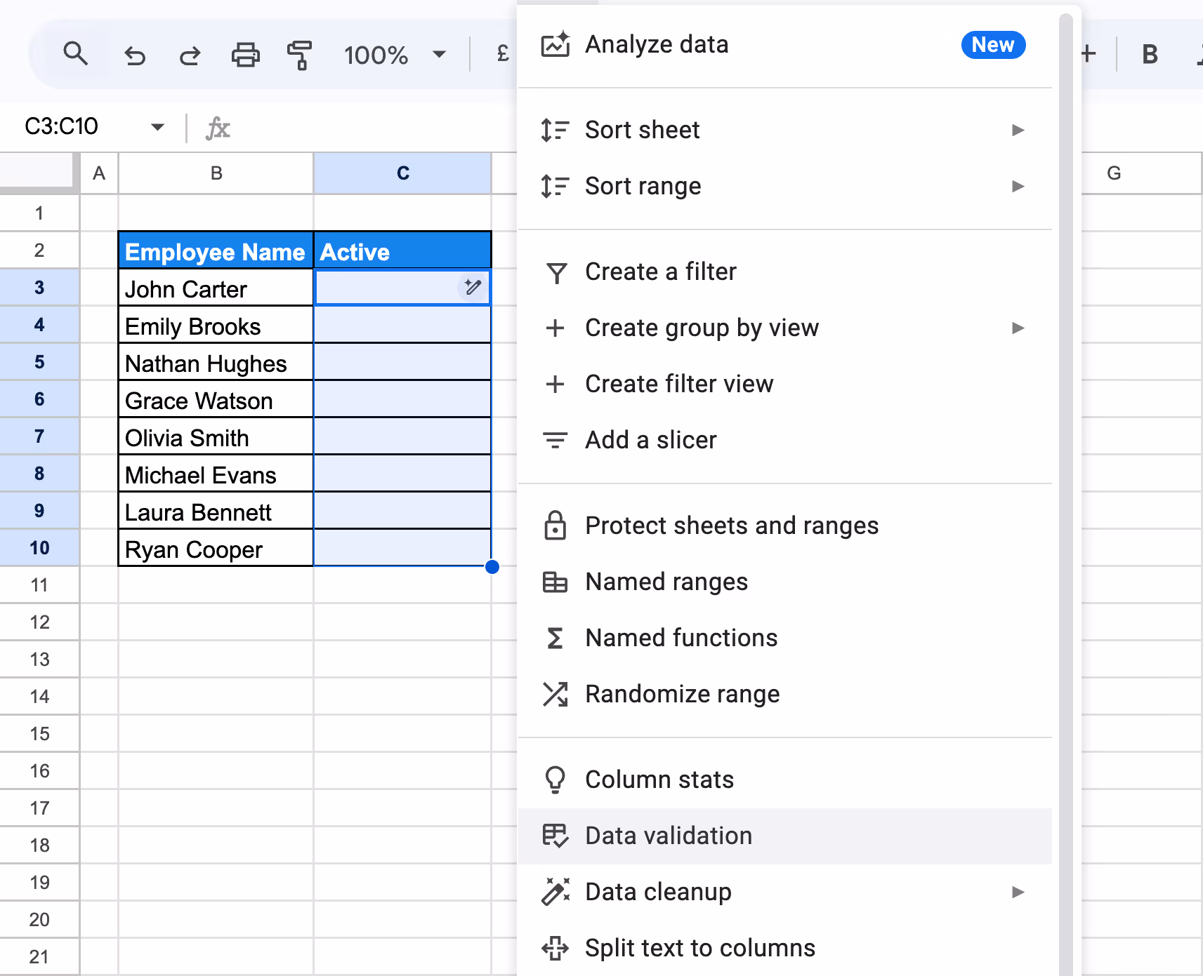
Step 2: Under Criteria, select the Checkbox from the dropdown options. 

Step 3: Choose Reject input to prevent users from typing anything else, and click Done to apply the rule.

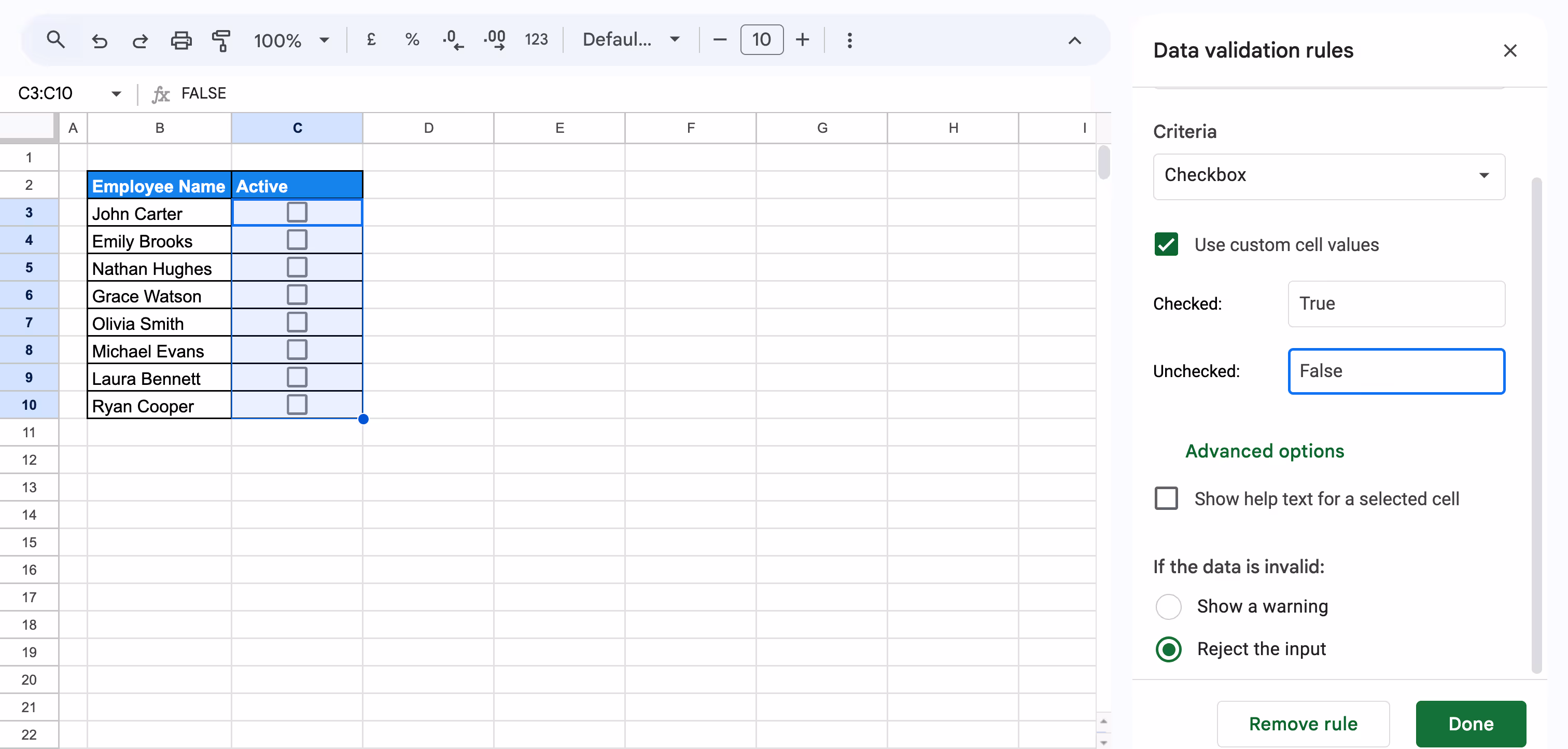
Now you can easily mark which employees are currently active.

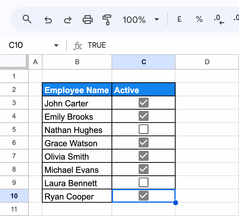
This ensures that only binary input is accepted, keeping employee status entries consistent and easy to use.

Advanced Data Validation Techniques to Use in Google Sheets 

Advanced data validation techniques help you handle more complex data entry needs. They’re useful for setting conditions, linking cells, and creating smarter, more dynamic spreadsheets in Google Sheets.

Implementing Custom Formula Validation

Custom formula validation in Google Sheets helps enforce specific rules that go beyond standard options. It's beneficial when working with key business data like sales targets, where accuracy matters.

Example:

Suppose you want to ensure the values entered in the Monthly Target column are always valid positive numbers – no negative amounts, text, or blanks.

Steps to apply custom formula validation:

Step 1: Highlight the cells in the Monthly Target column where you want the rule applied and click Data > Data validation to open the validation settings panel.

Step 2: Under the Criteria dropdown, select Custom formula is to create a custom logic rule. In the formula field, enter:

=AND(ISNUMBER(C3),C3>=0)

Here's what each parameter means:

• ISNUMBER(C3): Checks that the input is a number, not text or blank.
• C3>=0: Ensures the number is zero or higher.
• AND(...): Combines both checks, so the value must be numeric and non-negative.

Step 3: Choose Reject input to block any values that don’t match the rule, like negative numbers or text. Click Done to apply the rule and close the settings panel.

Test the rule by entering a negative number (like -1000) or text; it should show an error message.

This validation keeps your sales targets accurate and prevents invalid data from affecting reports or forecasts.

Using Conditional Formatting with Data Validation in Google Sheets 

Conditional formatting adds a visual layer to data validation, making it easier to spot important values or problems in your spreadsheet. It’s especially useful for highlighting data that needs attention.

Example:

Suppose you want to highlight active employees with a Lead Score below 5 in your dataset.

Steps to apply conditional formatting with data validation:

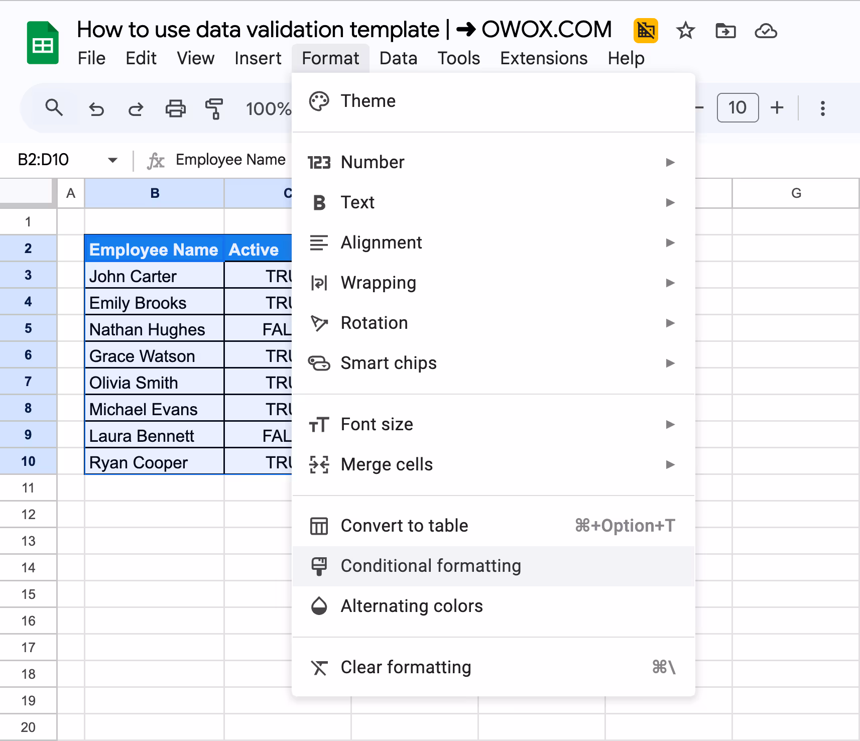
Step 1: Select the full range of rows where the Lead Score and Active status are recorded, and click on Format > Conditional formatting from the menu to open the formatting panel.

Step 2: Under “Format cells if,” choose Custom formula is and enter the following formula:

=AND($C2=TRUE, $D2<5)

Here's what each parameter means:

• $C2=TRUE Checks if the value in cell C2 is TRUE.
• $D2<5 Ensures the value in cell D2 is less than 5.
• AND(...): Combines both checks, so the condition is only TRUE if both are met.

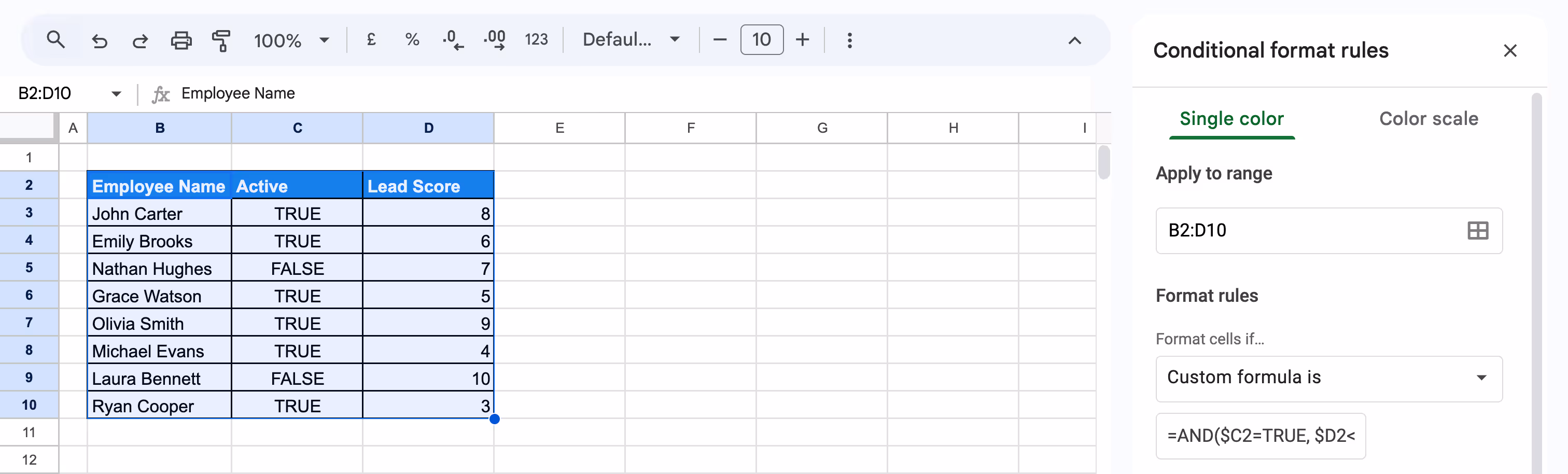
Step 3: Choose a formatting style, such as red fill or bold text, to make underperforming active employees stand out. Click Done to apply the rule to the range.

This method makes it easy to catch low lead scores at a glance while maintaining clean, validated data.

Implementing Conditional Data Validation Using the FILTER Function

Conditional Data Validation ensures that dropdown choices are filtered based on specific criteria, like employee status. This is useful when you only want to assign projects to active employees. 

Example:

Suppose you want to create a dropdown in the Assignee column that only shows employees with Active = TRUE, so inactive employees can't be selected for project tasks. The Main Sheet contains your complete employee data, including the Active status column.

Steps to apply conditional data validation with the FILTER function: 

Step 1: In a helper Sheet named “Filtered Data”, use the following formula to list only active employees:

=FILTER(B2:B10, C2:C10=TRUE)

Here's what each parameter means:

• B2:B10: This is the range of employee names that we want to filter.
• C2:C10=TRUE: This checks if each corresponding employee in the same row is marked as active (TRUE).
• FILTER(...): Returns only the employee names from B2:B10 where the active status in C2:C10 is TRUE.

Step 2: Select the filtered list, and name the range using the Name Box as ActiveList.

Go to the “Assignee” column in the main sheet where you want to apply the dropdown.

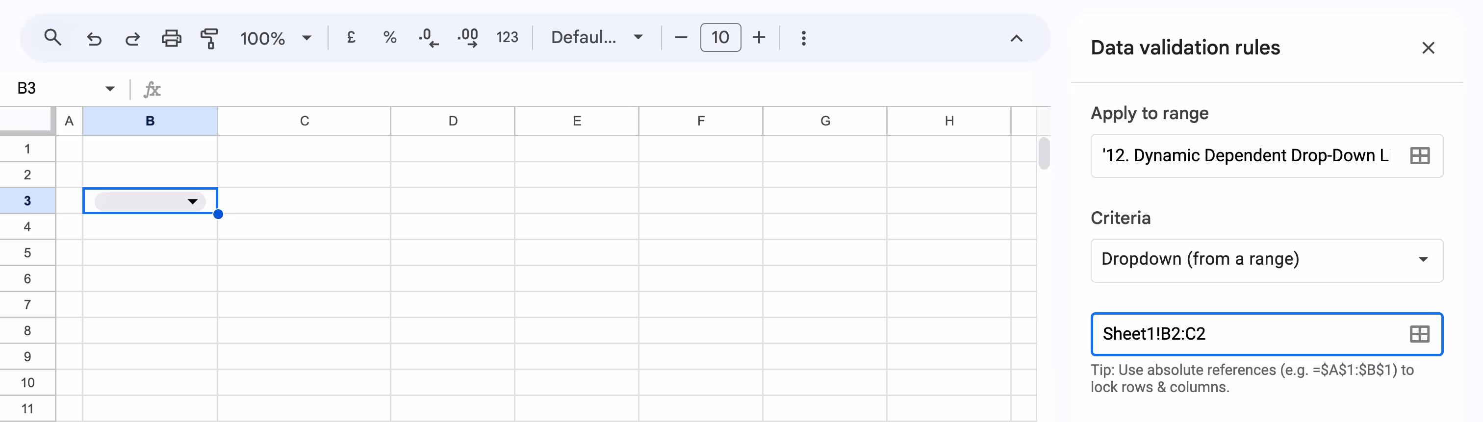
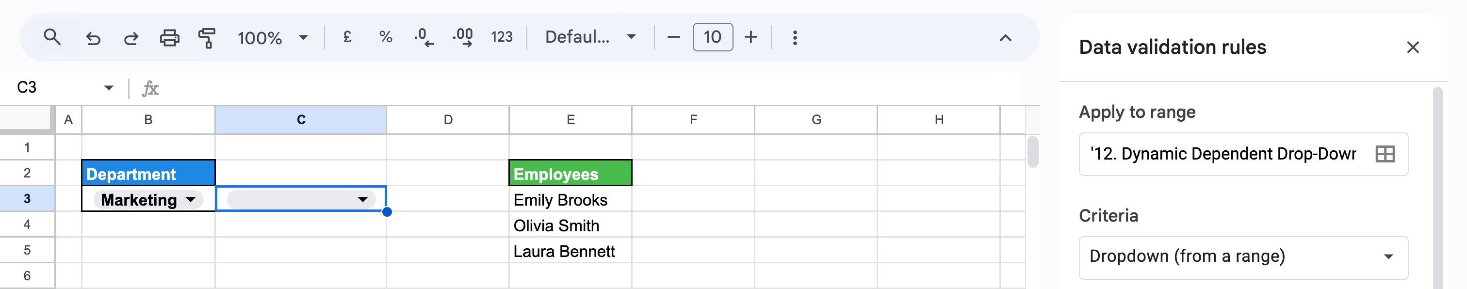
Step 3: Click Data > Data validation; for criteria, choose Dropdown (from a range) and enter the named range: ActiveList

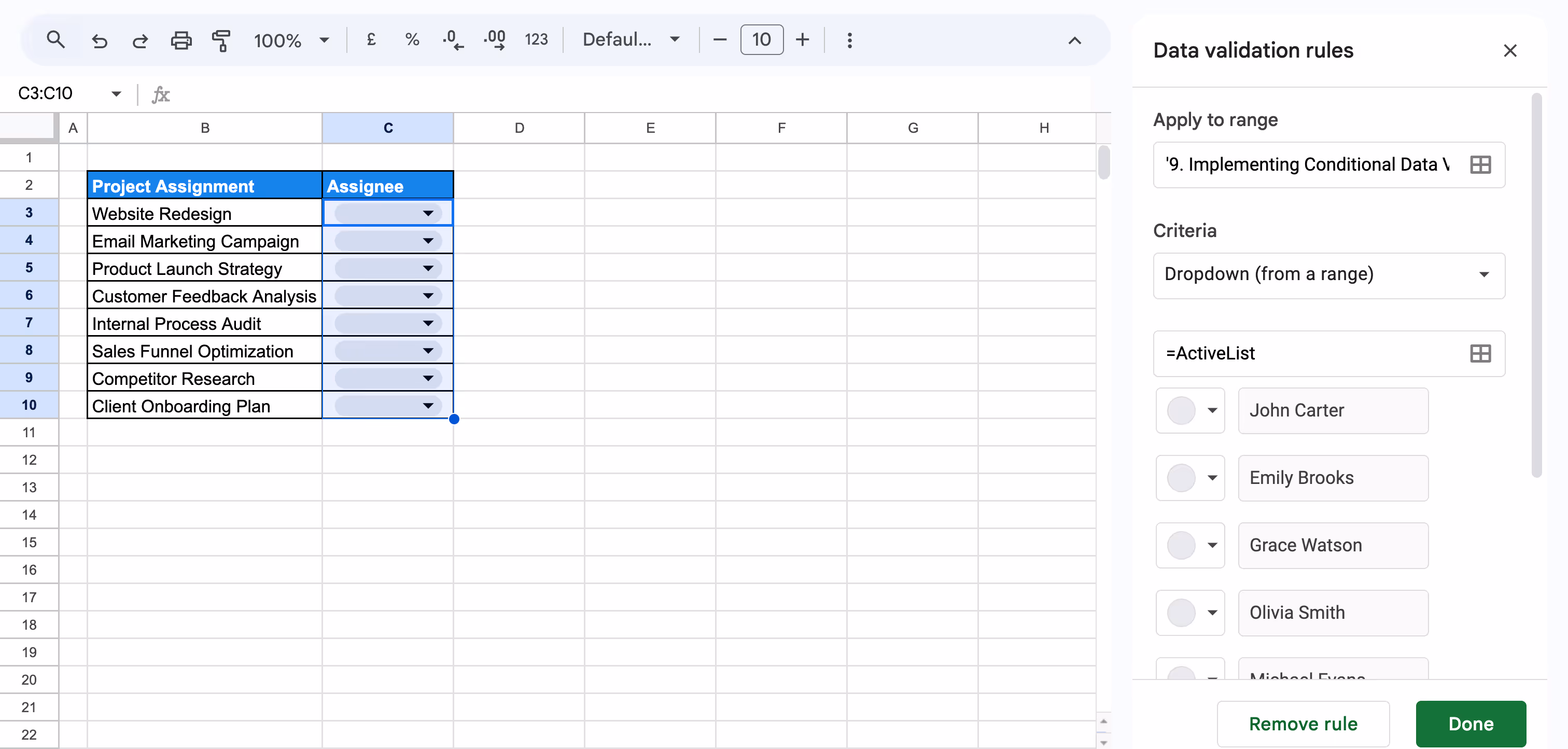
Step 4: Click on Done and click on the dropdown to assign the task.

Now, only employees marked as active can be assigned projects, ensuring accurate task allocation based on availability. 

Copying Data Validation Using the IMPORTRANGE Function

The IMPORTRANGE function helps you pull validated data from one Google Sheet into another. While it doesn’t copy the data validation rules themselves, it does carry over the clean, already-validated data – ideal for reporting or referencing from a central source.

Example:
Suppose you have a master dataset in another Google Sheet file, in a sheet named Main Sheet, and you want to pull the data from there into your current sheet. 

Steps to use the IMPORTRANGE function with validated data:

Step 1: Open the sheet where you want to display the department data and enter the formula below in a blank cell.

=IMPORTRANGE("https://docs.google.com/spreadsheets/d/1yg_eGNXY3AoRjBKU0PzPjxfGiGLG_rPCKj-ha5n_p5g/edit?gid=0#gid=0", "MainSheet!B2:C")

Here's what each parameter means:

• https://docs.google.com/spreadsheets/d/1yg_eGNXY3AoRjBKU0PzPjxfGiGLG_rPCKj-ha5n_p5g/edit?gid=0#gid=0: Link to the source file.
• MainSheet!B2:C: Range of data to import.
• IMPORTRANGE: Pulls the data into your current sheet.

When prompted, click Allow access to connect both sheets securely.

Step 2: The data from the Main Sheet will now appear in the new file. 

This imports clean department data from your main sheet while keeping it consistent across files.

Creating Dependent Dropdown Lists 

Dependent dropdown lists let you show different options based on another cell’s selection. It helps streamline data entry, especially when dealing with categories like regions, departments, or teams.

Dependent Dropdown Lists Using the INDIRECT Function 

Dependent dropdowns update one dropdown list based on the selection made in another. Using the INDIRECT function, you can easily link dropdowns without writing formulas in extra cells.

Example:

We’ll select a Department in one cell and use INDIRECT to display a list of matching employees in the next cell using named ranges.

Steps to create a dependent dropdown using INDIRECT:

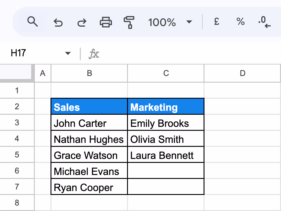
Step 1: In one sheet (Sheet1 in this example), set up the source data for your dropdowns. Use department names like “Sales” and “Marketing” as column headers in cells B2 and C2. Under each header, list the employees from your main data who belong to that department. This table will be used to create the dependent dropdowns using the INDIRECT function.

Step 2: Select the list under each department (e.g., B3:B for Sales) and name the range exactly as the header (e.g., Sales, Marketing) using Data > Named ranges.

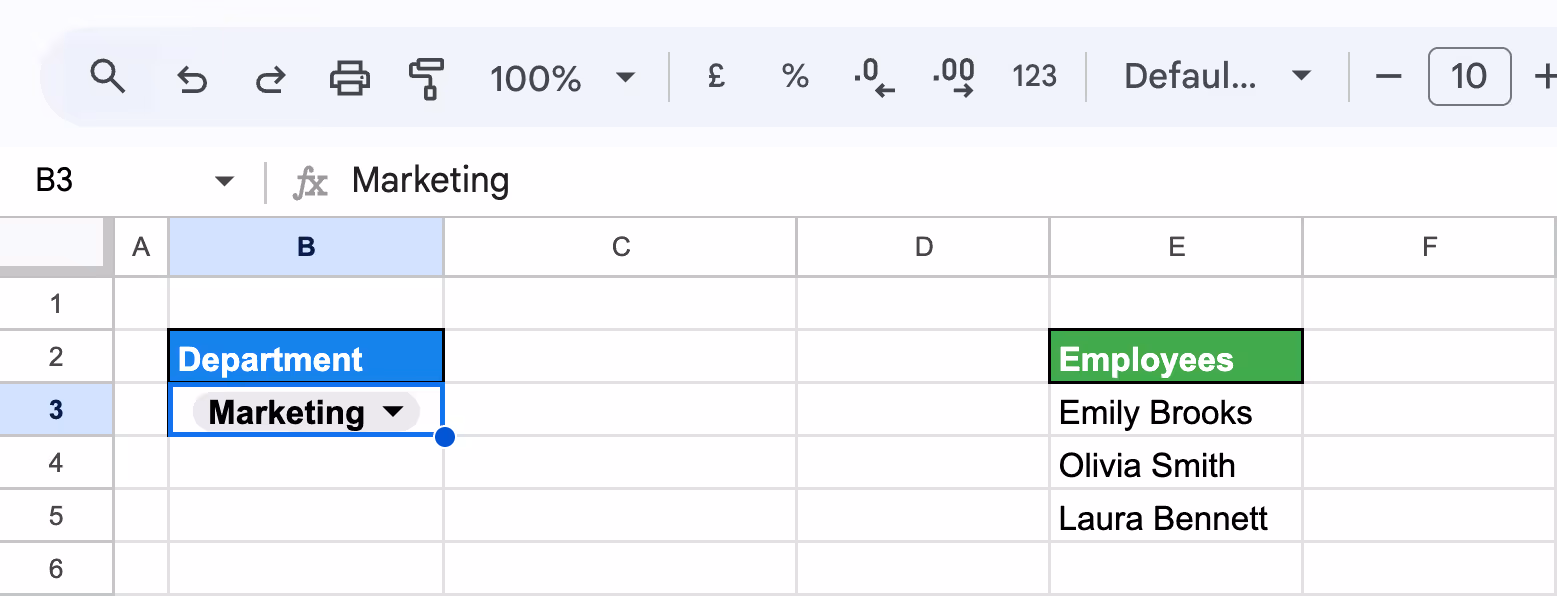
Step 3: In the tab where you want to place the dependent dropdown, click Insert > Dropdown on the respective cell and add the criteria as “Drop-down (from a range)”, then specify the Sheet and the departments (should match exactly with how you named the ranges).

Click Done to create the Department dropdown.

Step 4: Now, in the cell where you want the employee names to appear, insert the following function.

=INDIRECT(B3)

Click Done. This will show the list from the named range matching the selected department.

This method lets you build quick, flexible dropdowns without a helper – ideal for structured, repeatable selections.

Dynamic Dependent Drop-Down List Using XLOOKUP

Dynamic dependent dropdowns allow the values in one dropdown to automatically change based on the selection in another. This keeps your inputs relevant and clean, especially when categories like departments and roles are linked.

Example:

Suppose you're building a form where a user first selects a department, like 'Sales' or 'Marketing'. Based on that choice, the next dropdown should only display employees who work in the selected department.

Steps to create a dynamic dependent dropdown using XLOOKUP:

Step 1: In one sheet (Sheet1 in our example), organize your source data by adding department-based columns. Take the needed departments like “Sales” and “Marketing” as column headers, and list the corresponding employee names under each department. This structured layout will be used to create dynamic dropdown options later.

Step 2: In the sheet where you want the dropdown to appear, click Insert>Dropdown. Then choose Dropdown from a range under Criteria, and enter the sheet and column range where department names are stored (Sheet1!B2:C2 for our example)

Click Done to create the Department dropdown.

Step 3: In a different cell (in the same sheet), enter the following formula:

=TOCOL(XLOOKUP(B3, Sheet1!B2:C2, Sheet1!B3:C6), 1)

Here:

• B2: The list of departments (e.g., “Sales”, “Marketing”)
• Sheet1!B2:C2: The header row with department names
• Sheet1!B3:C6: The lists of employee names under each department
• TOROW(..., 1): Converts vertical data to a flat list and removes blanks

This will return a dynamic list of employees based on the selected department in B3. 

‍

Step 4: Go to the next cell, where you want the employee dropdown. Click Insert > Dropdown, choose Dropdown from a range, and type the range that contains the dynamic employee list returned by the XLOOKUP formula.

Click Done to apply the dependent dropdown.

This setup keeps dropdowns connected and auto-updated based on your selections.

Automating Data Validation with Google Apps Script

Google Apps Script allows you to automate dropdown lists and data validation across sheets, making your spreadsheet workflows faster and more scalable. This is useful when dropdown options depend on another sheet’s dynamic values.

Example:

Suppose you want to create an automated dropdown in the Assignee column of the sheet "Automating Data Validation with Google Apps Script" that only includes employees marked as Active = TRUE from the SourceSheet.

Steps to automate dropdown using Apps Script across sheets:

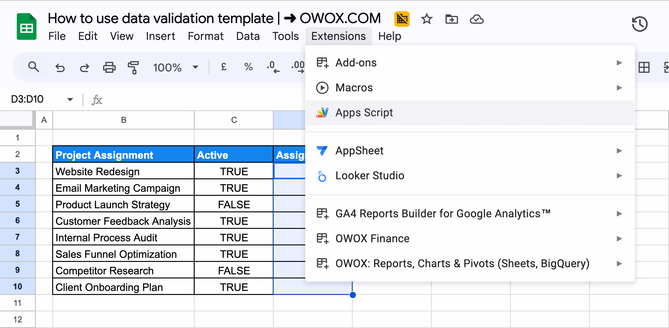
Step 1: Go to Extensions > Apps Script to open the Apps Script editor.

Step 2: Paste the following code in the editor:

1function updateAssigneeDropdown() {
2  const ss = SpreadsheetApp.getActiveSpreadsheet();
3  const sourceSheet = ss.getSheetByName('SourceSheet');
4  const targetSheet = ss.getSheetByName('Automating Data Validation with Google Apps Script');
5
6  // Get data starting from row 2 to account for headers in row 2
7  const sourceData = sourceSheet.getRange("B2:C9").getValues();
8  const header = sourceData[0]; // B2:C2
9  const nameIndex = 0; // Column B (Employee Name)
10  const activeIndex = 1; // Column C (Active)
11
12  // Get only employees marked as Active = TRUE
13  const activeEmployees = sourceData.slice(1) // skip header row
14    .filter(row => row[activeIndex] === true)
15    .map(row => row[nameIndex]);
16
17  // Apply validation to the Assignee column in project sheet (D3:D10)
18  const assigneeRange = targetSheet.getRange("D3:D10");
19  const rule = SpreadsheetApp.newDataValidation()
20    .requireValueInList(activeEmployees, true)
21    .setAllowInvalid(false)
22    .build();
23
24  assigneeRange.setDataValidation(rule);
25}

‍

Step 3: Save the script and click the Run button. Authorize the script when prompted.

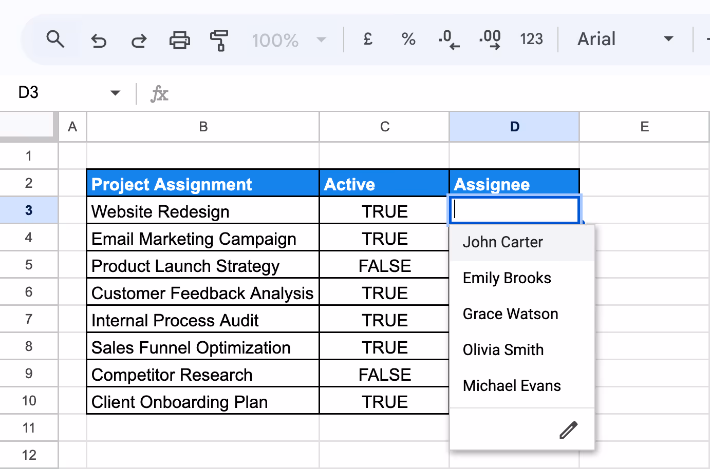
This will automatically update the dropdown list whenever employee statuses are edited in the SourceSheet.

Enforcing Character Restrictions Using REGEXMATCH in Data Validation

When you wish to limit what kind of text can be entered in a cell-like email domain or certain character patterns, REGEXMATCH is a great tool. It lets you validate input using custom text rules.

Example:
Suppose you want to restrict entries in the Email column to only accept addresses ending with @salescorp.com or @brandboost.co. or @marketlead.net.

Steps to Apply REGEX-Based Validation on the Email Column:

Step 1: Select the range of cells under the Email column in your dataset click on Data in the top menu, and choose Data validation. In the Criteria section, select Custom formula is, and enter the following formula:

=REGEXMATCH(C3,"@(salescorp\.com|brandboost\.co|marketlead\.net)$")

Here is what each parameter means:

• REGEXMATCH(C3, ...): Checks if the value in C3 matches the given pattern.
• @(salescorp\.com|brandboost\.co|marketlead\.net)$: Ensures the email ends with either @salescorp.com or @brandboost.co.
  
  • | means OR
  • \. escapes the dot, as dots have special meaning in regex
  • $ ensures the email ends with the given domain
    

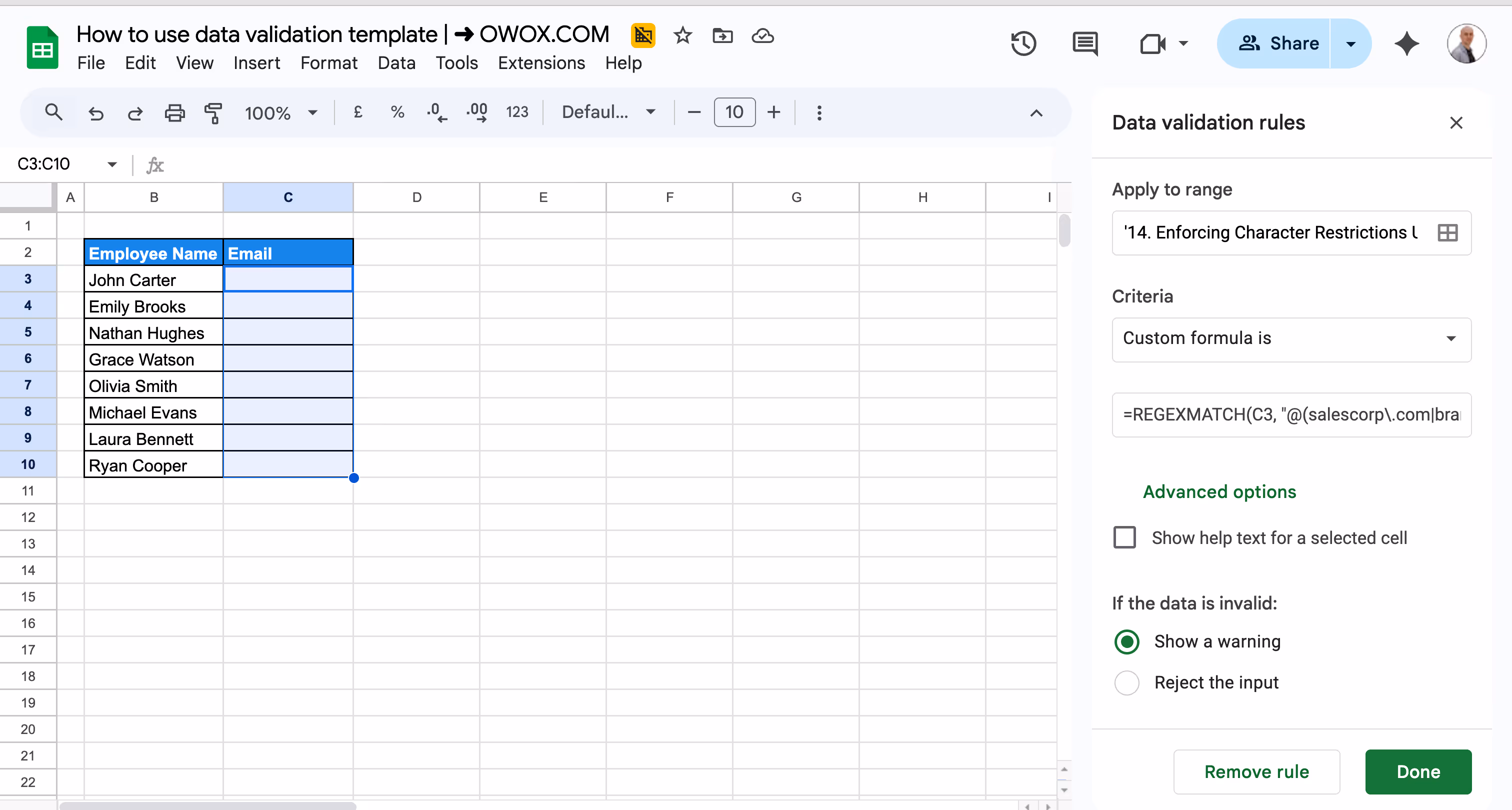
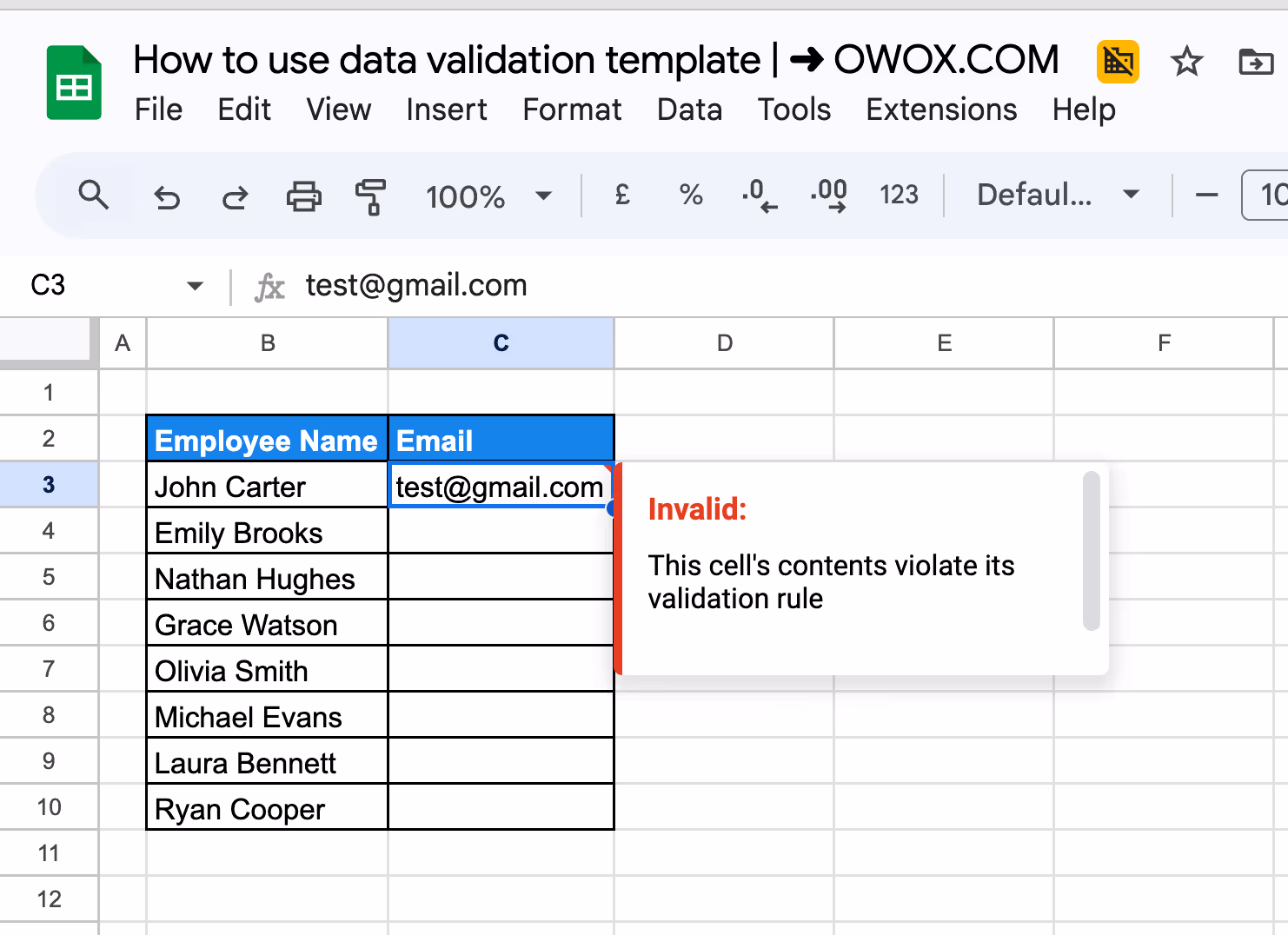
Step 2: Click Done to apply the rule. Test it by entering an invalid email, like test@gmail.com, and you’ll get a validation warning.

Only work-related email domains are accepted in the Email column, keeping your records consistent and secure. 

💡 Looking to enhance your data manipulation skills? Dive into our comprehensive guide on REGEX functions in Google Sheets. Learn how to efficiently search, extract, and replace text patterns to streamline your data analysis.​

Common Errors and How to Fix Them While Using Data Validation 

Even with the right setup, data validation can sometimes cause issues. Here are some common errors you might encounter and how to fix them quickly to keep your sheet running smoothly.

Violates Data Validation Rules Error

⚠️ Error: This appears when the entered value doesn’t match the set validation rule. It might be outside the allowed range, not part of a list, or incorrectly formatted. Even hidden spaces or characters can trigger this.

✅ Solution: Review the rule for accuracy. Remove extra spaces or formatting, especially from copy-pasted data. Try retyping manually and check formulas for possible issues or conflicts.

Data Validation Issues with Filtering & Sorting

⚠️ Error: Filtering or sorting your sheet can cause dropdowns or validation rules to break, especially if they rely on relative references or static ranges. This may lead to blank options or incorrect validations.

✅ Solution: Use absolute cell references (like $A$1) in your formulas. If you use named ranges, make them dynamic so they adjust when data is moved. You can also create helper columns to store original data and base your validation rules on those.

Overcomplicated Validation Rules

⚠️ Error: Applying too many rules or making them overly complex can confuse users. It slows down data entry and increases the risk of mistakes, especially if users don’t fully understand the requirements.

✅ Solution: Focus on key areas where validation matters most. Use simple, easy-to-follow rules and avoid layering too many conditions in one cell. Keeping it minimal helps users input data faster and more accurately.

Validation Errors Due to Strict or Unclear Rules

⚠️ Error: If your rules are too narrow or hard to understand, users may get blocked even when their input is reasonable. This leads to repeated frustration and incorrect entries.
✅ Solution: Loosen strict conditions where possible and provide clear guidance. Add help text or comments explaining the rule. Make sure your validation supports real-world input instead of blocking it unnecessarily.

Errors from Overlooking Edge Cases

⚠️ Error: Sometimes rules fail because they don’t account for special cases like leap years in dates or entries that are technically valid but rare. These can slip through during setup and cause errors later.

✅ Solution: Review your rules to catch possible exceptions. Test the validation with different scenarios and adjust to include edge cases. Being thorough from the start helps avoid problems later on.

User Errors Due to Lack of Guidance

⚠️ Error: Users might enter the wrong data simply because they aren’t sure what’s expected. If your validation doesn’t include help or hints, it’s easy for someone to make a mistake.

✅ Solution: Add input help text or comments explaining what kind of data is allowed. Even a short note can make a big difference. Clear instructions reduce confusion and improve the quality of entries.

Best Practices for Data Validation in Google Sheets 

Using data validation effectively isn’t just about setting rules. Following a few best practices can help keep your data clean, user-friendly, and reliable, especially when working with others.

Highlighting Errors with Conditional Formatting

Pairing data validation with conditional formatting helps you catch errors visually. For example, you can automatically highlight cells in red when someone enters invalid data. 

This makes mistakes easy to spot at a glance, especially in large spreadsheets. It’s a helpful way to guide users and ensure that incorrect entries don’t go unnoticed or get buried in the data.

Keeping Validation Lists Updated

If you're using dropdown lists or value ranges for data validation, keep those lists up to date. Over time, your data may change, new options might be needed, or old ones removed. 

If the list isn’t updated, users might choose incorrect values or get confused. Regular updates keep your validation relevant and your data clean and consistent.

Test Validation Rules Before Implementation

Before applying validation rules across your sheet, especially if it’s shared, test them first. Try entering both valid and invalid inputs to make sure the rules respond correctly. 

Testing helps catch unexpected behavior or overly strict conditions. It’s a small step that prevents frustration later and ensures the validation works smoothly for everyone using the sheet.

Documenting Validation Rules for Reference

Create a dedicated section or sheet in your document to list all your validation rules. This is helpful when someone new works on the sheet or if you need to explain how it works. 

It also saves time when you revisit the spreadsheet later and need to remember why a certain rule was set up. Clear documentation makes your spreadsheet easier to manage, especially in team or long-term projects.

Regularly Reviewing and Updating Validation

Your data needs can change over time, and your validation rules should change with them. A rule that worked six months ago might not make sense today. Make it a habit to review your rules regularly. 

This helps ensure your spreadsheet stays accurate, easy to use, and aligned with your current goals or workflow. Setting regular check-ins can prevent outdated rules from causing issues down the line.

Gathering User Feedback on Validation Rules

If others are entering data into your sheet, ask them how the validation rules are working for them. They might find parts that are confusing or suggest ways to make input easier. 

User feedback is valuable for improving your setup and ensuring the rules are practical, not just technically correct. Simple changes based on user input can lead to better accuracy and smoother collaboration.

Using Advanced Functions to Search and Work with Data in Google Sheets

Google Sheets offers powerful functions that go beyond simple filters or searches. These advanced tools make it easier to find, analyze, and work with the right information, especially when dealing with large datasets. By applying logic-based formulas, you can automatically surface relevant details without manually scanning through rows.

• SEARCH: Finds the position of a specific text string within another. Useful for identifying if certain keywords or values are present in a cell.
• SUM: Adds together a range of numbers, making it ideal for calculating totals like sales, targets, or budgets across rows or columns.
• AVERAGE: Calculates the mean of a group of numbers. Perfect for analyzing performance metrics like average lead score or monthly targets.
• CONCATENATE: Combines multiple text strings into one, simplifying the process of merging data from different cells or sources.
• VLOOKUP: Searches for a value in the first column of a range and returns a corresponding value from another column. Useful for matching names to departments or roles.
• QUERY: Allows you to filter, sort, and display data using SQL-like syntax. It’s powerful for extracting specific information from large datasets quickly.

Boost Your Data Analysis with OWOX: Reports, Charts & Pivots Extension

Take your data analysis to the next level with the OWOX Reports. It’s designed to help you quickly create clear, visual reports from your Google Sheets data. No need to build complicated formulas or spend extra time formatting charts manually. OWOX does the heavy lifting for you.

Whether you're tracking sales, performance, or project updates, OWOX makes it faster to spot trends and share insights. Install the extension and start building visual dashboards in just a few clicks – all directly from your spreadsheet.