Why your scheduled refresh keeps wiping Google Sheets formulas (and how to fix it)
A scheduled refresh does not wipe a spreadsheet at random: it rewrites the block of cells it owns, and anything typed inside that block goes with it. This guide shows which cells an OWOX Data Marts report to Google Sheets owns and which it leaves alone, five patterns that keep formulas alive through every refresh, what a #REF! after a refresh means, and a short note to forward to the person whose column disappeared.

“The margin column I added is gone again.” If you set up the scheduled export into that spreadsheet, this message lands on you the morning after the refresh, usually from someone who has rebuilt the same column three times. The refresh did not break the sheet at random. It rewrote the block of cells it owns, and the formula was sitting inside that block.
So the fix is mostly about placement: which cells an OWOX Data Marts report owns, which it never touches, and five Google Sheets patterns that keep formulas, totals and lookups alive. The last section is a plain-words note for the person whose column disappeared.
Product behaviour below is quoted from the Google Sheets destination documentation, functions from Google’s help pages. The patterns were written from that documentation, not tested in a live spreadsheet.
Why the refresh wipes your formulas
Why the refresh wipes your formulas
A scheduled report cannot ask anyone which cells they meant to keep, so every reporting tool decides which cells it owns. Whatever sits inside that area is replaced on the next run, whether it is a value, a note or a formula.
You can find that boundary in a minute with any tool. A report writes only to the tab it was set up for (in OWOX Data Marts, the tab whose link you pasted into the report), so a copy of the spreadsheet is never refreshed. Point a test report at a test tab, or use the real tab at a quiet time after saving a copy as a backup. Type an X in four places: inside the data, just under the last data row, in the first empty column to the right, and on another tab. Run the report once. The X’s that survive mark the space that is yours.
In OWOX Data Marts the owned area is called the imported range: every cell from row 1 down to the last data row, across the columns that came from the Data Mart. The documentation is blunt about what happens inside it:
- Headers in row 1 are rewritten to the latest column names or their aliases. Renaming a header cell by hand does not stick.
- Data cells are replaced by the values from the latest run. A formula typed into an imported column “disappears on the next refresh – even when SQL returns NULL for that cell”.
- Cells in the imported columns below the last data row are cleared. When a run returns fewer rows than the last one, the leftover rows are wiped, so nobody reads last week’s numbers under this week’s. A totals row typed under the data goes the same way.
The row count changes on every run, so there is no safe row below the data. The safe direction is to the right, and the safe place for totals is another tab.
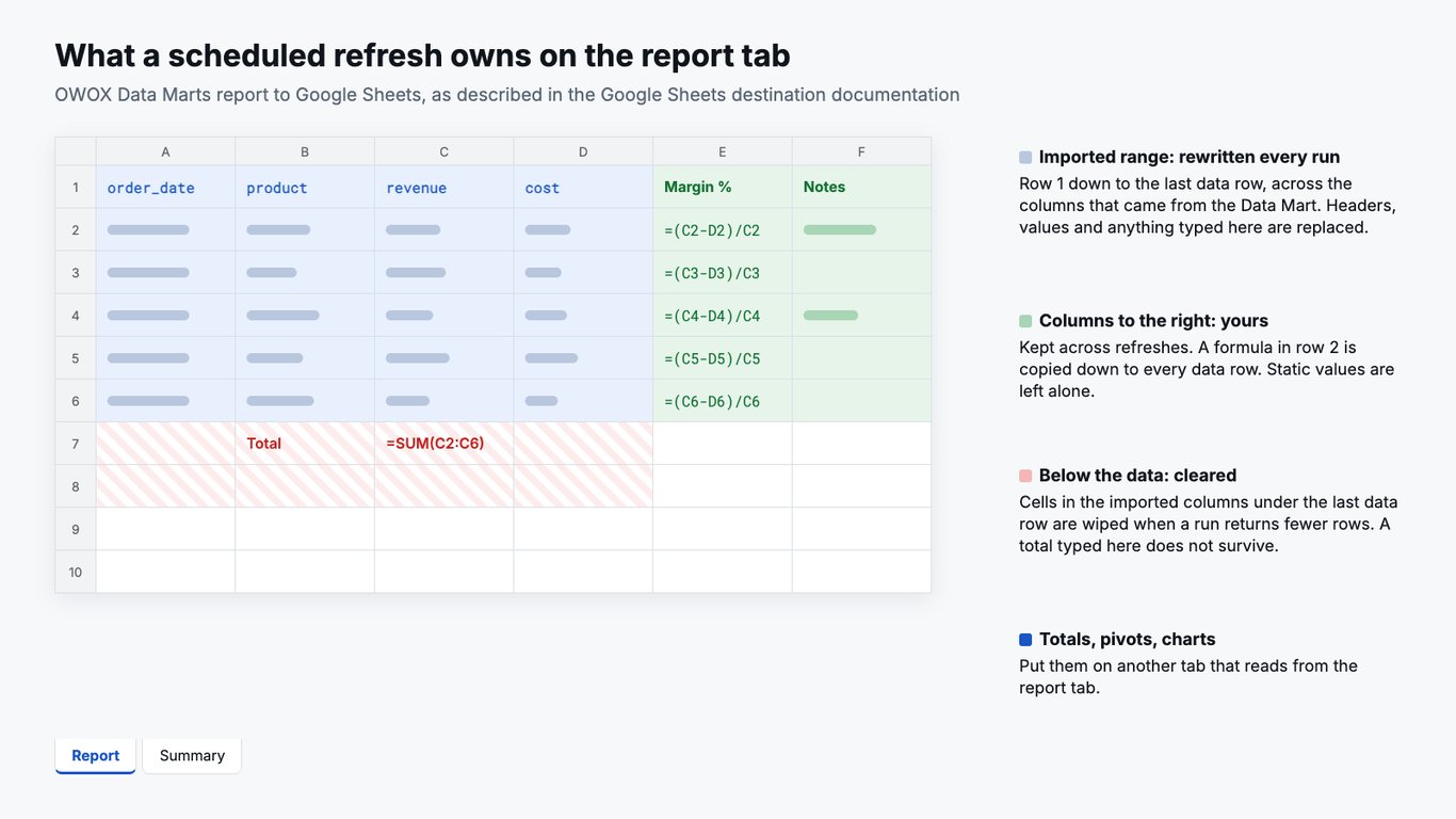
What survives a refresh, and what does not
What survives a refresh, and what does not
Everything outside the imported range is yours. The documentation spells out what that means:
| You did this | What the next refresh does |
|---|---|
| Typed a formula or a value into an imported column | Replaces it |
| Put a formula in a column to the right of the imported range | Keeps it |
| Wrote a formula in row 2 of a column to the right | Copies it down to every data row, shifting relative references the way the fill handle does |
| Typed static values (notes, a lookup table) in a column to the right | Keeps them: fill-down only acts where row 2 holds a formula |
| Dragged the imported columns into a different order | Keeps your order and writes each column by its name |
| Built a pivot table, chart or named range on the imported range | Keeps it working: columns are added and removed with Sheets’ own insert and delete |
| Put a total under the last data row | Clears it, if it sits in an imported column |
| The run failed before any data was delivered | Leaves the sheet exactly as it was |
Two caveats. Columns are matched “by their SQL name, not by position”, so a column renamed in the SQL counts as a new one (see below). And a failed run is only harmless before delivery: “If the failure happens after OWOX has started updating the sheet, the sheet can be left partly updated until the next successful run.” Check Run History before you trust a sheet after a failed run, or, without access to OWOX, the refresh time in the note on the first header cell (pattern 5).
OWOX Data Marts
See your first report built in real time. 15 minutes.
- Connect your data warehouse
- Pick your metrics
- Get a live Google Sheets report
In the time it takes to write a ticket. Then imagine never writing that ticket again.
Book a DemoWe'll use your actual use case
Five patterns that keep formulas alive
Five patterns that keep formulas alive
Most “my formula vanished” messages come down to one of these five. The first two are about where things go, the other three about how formulas point at data that changes shape every morning.
1. Calculate to the right, and write the formula once in row 2
Say the report writes four columns: order_date, product, revenue, cost. The first empty column to the right is yours. Put a header in row 1, say Margin %, and one formula in row 2:
=IF(C2=0, , (C2-D2)/C2)On the next refresh OWOX copies it down to every data row, the way the fill handle would. Nobody drags formulas after a refresh any more, and when this month has more rows than last month, the new rows get the formula too. This is on by default; there is nothing to configure.
The documentation says the row-2 formula is extended “to every data row”. It does not promise that a value typed lower in the same column survives, so treat the whole column as the formula’s and never type over rows 3 and below. A number you type yourself, such as a monthly target, gets a column of its own: fill-down skips any column whose row 2 holds a value rather than a formula. Say F2 holds the target. In the next column, % to goal is =C2/$F$2: the dollar signs lock F2, so every copied row divides by the same cell.
If the Data Mart gains a column, it is appended at the right edge of the imported range and your Margin % column shifts right by one; references to it shift too, as with any inserted column.
2. Keep the report on its own tab, and summarise on another
Totals, pivot tables, charts and the numbers someone pastes into a slide belong on a second tab, say Summary, that only reads from the report tab.
This is the pattern most people mean by “a second tab to keep formulas”. Within one spreadsheet it needs no special function: a plain reference such as Report!C2:C100000 reads the other tab (pattern 4 explains the bound). IMPORTRANGE is for reading from a different spreadsheet, which is pattern 5’s job.
3. Find columns by header name, not by letter or number
This is the failure that sends wrong numbers upward without an error. A lookup such as =VLOOKUP(A2, Report!A:F, 6, FALSE) reads “the sixth column” of the range. That 6 is a number, not a reference, so nothing updates it when the columns change: a column added by the report, a renamed one moved to the right edge, or a column someone dragged. The formula keeps working and quietly returns whatever now sits sixth.
Look the column up by the header people see in row 1 instead. INDEX and MATCH can find both the row and the column; Google’s own example makes “both row number & column number” dynamic. Here is the VLOOKUP above, rewritten to find revenue by its header:
=IFERROR(INDEX(Report!A1:Z100000,
  MATCH(A2, Report!A1:A100000, 0),
  MATCH("revenue", Report!A1:Z1, 0)),
  "header not found")
MATCH with 0 asks for an exact match. Both ranges span columns A to Z, so the position MATCH returns is the column INDEX reads. IFERROR turns a missing header into a visible message instead of #N/A on someone’s summary. A total works the same way, with row 0 returning the whole column: =IFERROR(SUM(INDEX(Report!A1:Z100000, 0, MATCH("revenue", Report!A1:Z1, 0))), "header not found").
XLOOKUP is shorter: =XLOOKUP("revenue", Report!A1:Z1, Report!A2:Z100000) returns the revenue column, and LET can name it once if a formula uses it several times. Search for the column name you see in row 1, which may differ from the name in the query. Two things to avoid: INDIRECT, because an address written as text ("Report!C2:C100000") does not move when columns are inserted or deleted; and converting the imported range into a Sheets table, which the OWOX documentation does not cover, so keep it a plain range. See also INDEX and MATCH in Google Sheets.
4. Size ranges for growth, then use FILTER and QUERY on the Summary tab
The row count changes on every run, so a range cut at today’s last row (C2:C500) silently misses new rows. An open-ended range (C2:C) never misses one, but the OWOX documentation names whole-column reads from other sheets, like COUNTIF('My report'!N:N, …), as a reason a refresh can fail: each change triggers a recalculation of every formula that reads the sheet. Its advice is to “limit the formulas to the rows they need – N2:N100000 instead of N:N”.
So: bound ranges well above the largest result you expect, such as row 100000, inside SUM, MATCH and lookups, which read the range and return one value. Formulas that return a value for every row are different. An ARRAYFORMULA over C2:C100000 fills all 100,000 rows, blank or not, and recalculates them. For row-by-row output, FILTER returns only the rows that hold data, and handles arrays by itself:
=FILTER(Report!C2:C100000 - Report!D2:D100000,
  Report!C2:C100000 <> "")
QUERY does group-and-sum in one cell: revenue by product, for instance.
=QUERY(Report!A1:D100000,
  "select B, sum(C) where B is not null
   group by B", 1)
Three limits are worth knowing. QUERY names the columns of a range by their letters (B, C), so it reads whatever sits there: if your team rearranges the report tab, rewrite the query. QUERY also gives each column one type, the majority one, and treats the rest as empty, so a column of product codes such as 00123 mixed with plain numbers can lose values without an error. And keep array formulas off the report tab: fill-down copies a row-2 formula to every row, and a formula that already fills the column by itself does not belong there. Our guides to QUERY and array formulas go deeper.
5. Put a warning on the imported columns, and split heavy workbooks
Most lost formulas were typed into an imported column by someone who did not know it. Two things help:
- Read the header note. Each imported header carries a note ending in
--- Imported via OWOX Data Marts ---, and the first one also shows the Data Mart name, the time of the last refresh and a link to the report. Hover it before you edit a column. - Add a warning. In Google Sheets, Data → Protect sheets and ranges on the imported columns, with Show a warning when editing this range, asks anyone who types there to confirm. If you choose Restrict who can edit this range instead, keep the Google account or service account the report writes with on the list, or you are locking out the report itself.
For a heavy workbook, the OWOX documentation suggests delivering the report to a separate spreadsheet and bringing the values you need in with IMPORTRANGE. Google’s IMPORTRANGE guidance adds: limit receiving sheets, avoid chains, and “restructure and condense your result” first. So import a few aggregated rows, not every record:
=IMPORTRANGE(
  "https://docs.google.com/spreadsheets/d/…",
  "Summary!A1:C50")
The first time a spreadsheet pulls from a new source, Google asks you to grant it permission; after that it updates on its own. See how to use IMPORTRANGE for the syntax.
Why formulas show #REF! after a refresh
Why formulas show #REF! after a refresh
A #REF! right after a refresh usually means a column in the Data Mart went away:
- A removed column is deleted from the imported range, and “user formulas that referenced the removed column become #REF! – an honest signal that the column they depended on is gone.”
- A renamed column is treated as removing the old one and adding a new one. Formulas on the old column become #REF!; repoint them to the new one at the right edge of the imported range.
An error beats a formula that quietly reads the wrong column. If you only want a friendlier header, do not rename the column in the SQL. Set a display alias in the Data Mart’s Output Schema: the alias “appears in row 1 of the destination sheet without inserting or deleting any columns”. Matching still uses the SQL name, so nothing downstream breaks.
When you rename or remove a column on purpose, tell the people who build on that sheet first. A header lookup (pattern 3) for the old name returns “header not found”, which is fixed by changing one name.
The silent case needs a check of its own. Before numbers from the sheet go to anyone:
- The refresh is today’s: hover the first header cell; its note shows the time of the last refresh.
- The headers are the ones your formulas expect: no cell says “header not found”.
- A total ties: select the revenue column on the report tab; the sum Sheets shows in the bottom-right corner should equal the Summary total.
- One row you know looks right: a recent order, a product you can check elsewhere.
How to schedule the refresh in OWOX Data Marts
How to schedule the refresh in OWOX Data Marts
The data travels source to warehouse to sheet: an analyst defines a Data Mart on your warehouse, and a report writes it to a Google Sheets tab on a schedule. More in .
In OWOX Data Marts Cloud, with a Google account signed in through OAuth: add a Google Sheets destination with Connect Google Account (a service account JSON key is the documented alternative for unattended workflows; see destinations). On the Data Mart’s Destinations tab, click + New Report and paste the link to an empty target tab; it must include the tab’s gid. On the Triggers tab, add a Report Run trigger, daily, weekly, monthly or at an interval. The report trigger does not wait for the data import, so schedule it after the import usually finishes, and watch the first runs in Run History.
A note for the person whose column disappeared
A note for the person whose column disappeared
If someone asked you why their work keeps vanishing, this part is for them. Copy it and send it, but fill in every bracket first: an unfilled note leaves them guessing which columns are theirs.
Nobody did anything wrong: the area the report rewrites just was not marked. The [Orders] tab is refreshed automatically every [morning at 7]. The refresh rewrites columns [A to D], from the header row down to the last row of data, and clears anything below the data in those columns. Anything typed there, including formulas, is replaced.
Your own work is safe anywhere to the right of column [D]. Write a formula once in row 2 of an empty column, and it copies itself to every row after the next refresh. Numbers you type yourself, such as targets, are safe to the right too, in a column of their own. In a formula that divides by a target, lock the cell with dollar signs, such as =C2/$F$2, so it stays put as the formula copies down. Put totals, charts and pivot tables on the [Summary] tab, not under the data.
Before you send numbers on, hover the first header cell: the note shows when the data was last refreshed. Check one row you know. If a cell shows #REF! or “header not found” after a refresh, a column in the report was renamed or removed. Send me the cell, and I will tell you what changed.
Turn your data into decisions.
Governed data marts give you the clean foundation ML needs to actually work.
- No AI hallucinations
- Analyst-governed definitions
- Every number traces to SQL
Frequently Asked Questions
Why does my scheduled data refresh overwrite formulas in Google Sheets?
A scheduled report owns a block of cells and rewrites it on every run. In OWOX Data Marts that block is the imported range: every cell from row 1 down to the last data row, across the columns that came from the Data Mart. A formula typed into one of those columns is replaced on the next refresh, even when the source returns an empty value. Put your formulas in columns to the right of the imported range, which the refresh keeps (Google Sheets destination documentation).
Where can I put formulas so a refresh does not delete them?
In any column to the right of the imported range, or on another tab. In OWOX Data Marts, a formula written in row 2 of a column to the right is copied down to every data row on the next refresh, and static values in those columns are left alone. Totals, pivot tables and charts belong on a separate tab that reads from the report tab (Google Sheets destination documentation).
Why do my formulas show #REF! after a scheduled refresh?
A column they referenced was removed from the Data Mart, or renamed: OWOX Data Marts treats a rename as removing the old column and adding a new one at the right edge of the imported range. Repoint the formula to the new column. To change only the header people see, set a display alias in the Data Mart's Output Schema instead: the alias appears in row 1 without inserting or deleting any columns (Google Sheets destination documentation).
Why did the totals row under my imported data disappear?
Cells in the imported columns below the last data row are cleared on every refresh, so a run with fewer rows never leaves old numbers under new ones. That clears a totals row typed under the data, too. Calculate totals on a separate tab instead, for example with =SUM(Report!C2:C100000) (Google Sheets destination documentation).
Can I rearrange the columns of an imported report in Google Sheets?
Yes. If you drag the imported columns into a new order, OWOX Data Marts remembers it on the next refresh and writes each column into your layout, matching columns by their SQL name, not their position (Google Sheets destination documentation). Formulas that refer to a column by its letter can still point at the wrong column after a reorder, so look columns up by header with INDEX and MATCH.