How to use INDEX MATCH in Google Sheets: formula, examples and errors

Exploring the INDEX function

INDEX returns the value of the cell at a given row and column of a range.

Syntax of INDEX function

The syntax of the INDEX function in Google Sheets is:

=INDEX(reference, [row], [column])

Let’s break it down:

• reference: the range to take the value from.
• row (optional): the row number, counted from the top of the range.
• column (optional): the column number, counted from the left of the range.

Example of INDEX function

To get the value in the eighth row and second column of the range B3:D11:

=INDEX(B3:D11, 8, 2)

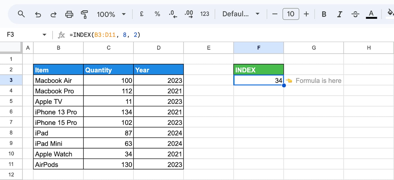
The function returns 34. The row and column are counted inside the range, not on the sheet: the eighth row of B3:D11 is row 10 of the sheet.

Understanding the MATCH function

The MATCH function searches a single row or column for a value and returns its position in that range.

Syntax of MATCH function

The syntax of the MATCH function in Google Sheets is:

=MATCH(search_key, range, [search_type])

Let’s explain:

• search_key: the value to find.
• range: the row or column to search. It must be one-dimensional.
• search_type (optional): 0 for an exact match; 1 (the default) when the range is sorted in ascending order; -1 when it is sorted in descending order.

For lookups by name or ID, always write the 0. Without it, MATCH assumes sorted data and can return the position of a different item without any error.

Example of MATCH function

To find the position of “iPad” in the range B3:B11:

=MATCH("iPad", B3:B11, 0)

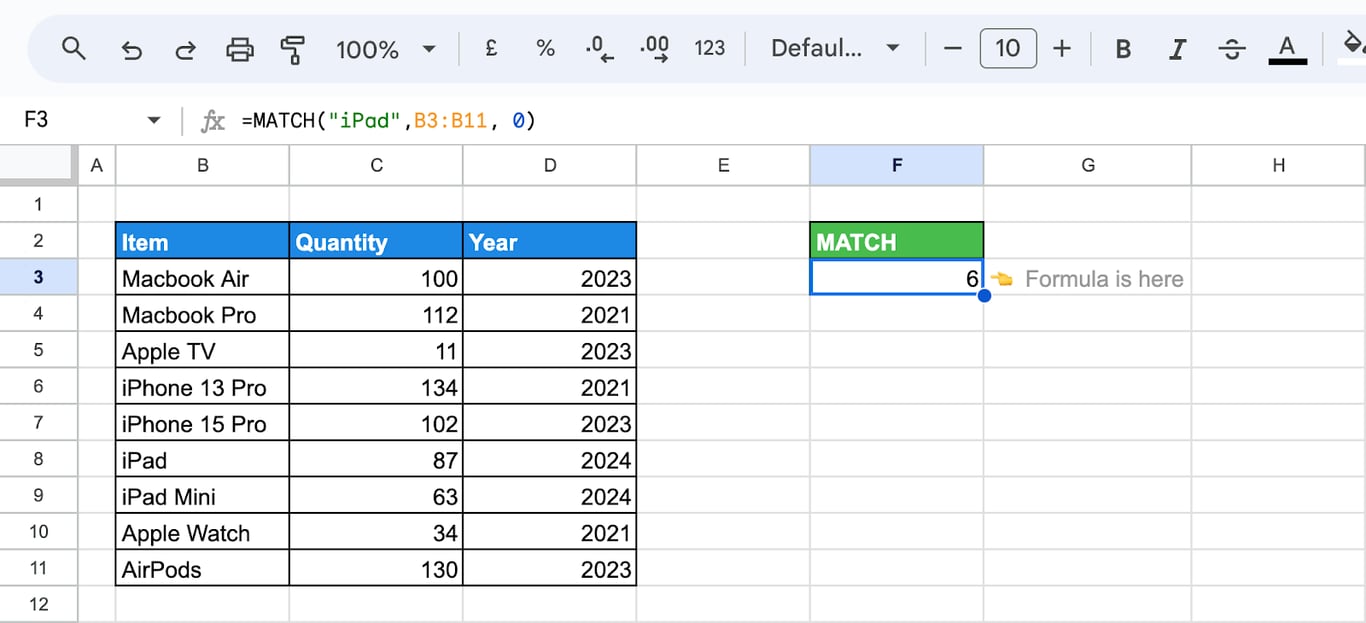
“iPad” is in cell B8, the sixth cell of the range, so the function returns 6.

INDEX MATCH or VLOOKUP?

Both return the same result for a simple lookup. INDEX MATCH is the better choice when:

• The value to return is left of the lookup column. VLOOKUP only looks to the right of its first column.
• Columns get inserted or moved. VLOOKUP counts columns by number, so a new column shifts the result. INDEX MATCH points at the return column directly. On a tab that a scheduled report rewrites, look the column up by its header instead, as shown in why a scheduled refresh wipes Google Sheets formulas.
• You need more than one condition, or a case-sensitive match.

💡 For a lookup to the right on a stable table, VLOOKUP is shorter to write. See our guide to VLOOKUP in Google Sheets. Google Sheets also has XLOOKUP, which covers both cases in one function; see XLOOKUP vs VLOOKUP.

How to use INDEX MATCH step by step

The example looks up the quantity of each item listed in column F in the table B3:D11.

Step 1: Identify the lookup range and selection criteria

Decide on three things: the lookup value, the column to search and the column to return.

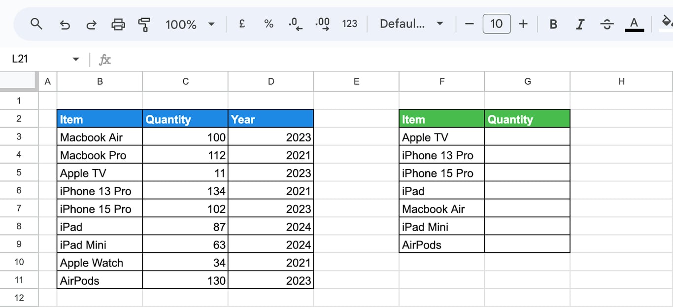
The item names in column F are the lookup values, starting with ‘Apple TV’ in F3. The table is B3:D11: the names are searched in column B, and the quantity is returned from the second column of the table.

Step 2: Implement the MATCH function to locate data

Select the cell for the result and type =MATCH(. The first argument is the lookup value, cell F3.

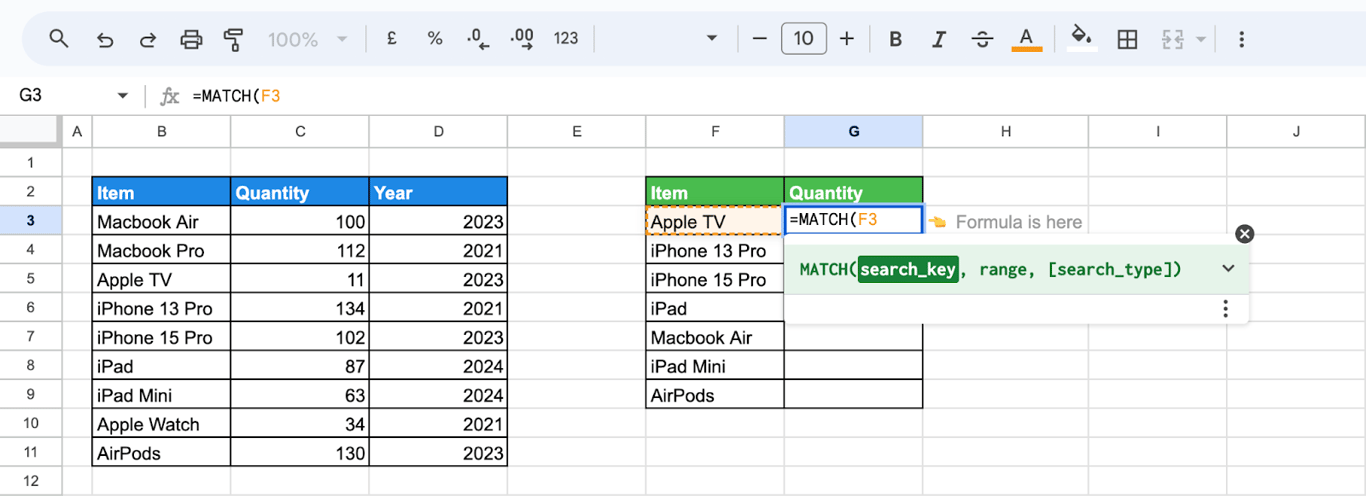
The second argument is the column to search, B3:B11. It has to be a single column; a range of several columns returns #N/A.

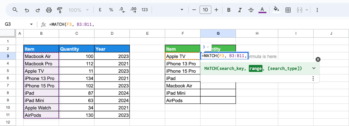
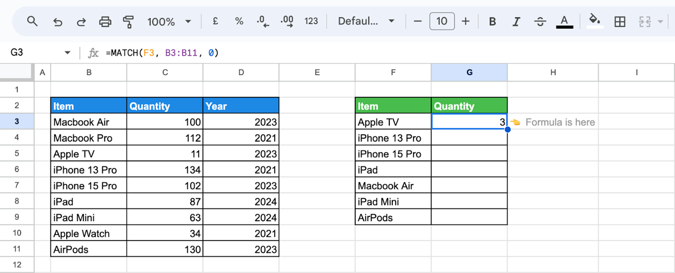
The third argument is the search type: 0 for an exact match.

The formula returns the position of the item in the column:

=MATCH(F3, B3:B11, 0)

Step 3: Wrap MATCH function with INDEX function

Put the MATCH inside INDEX:

• First argument: the table to return a value from, B3:D11.
• Second argument: the MATCH from step 2, which supplies the row number.
• Third argument: the column of the table to return, here 2 for the quantity.

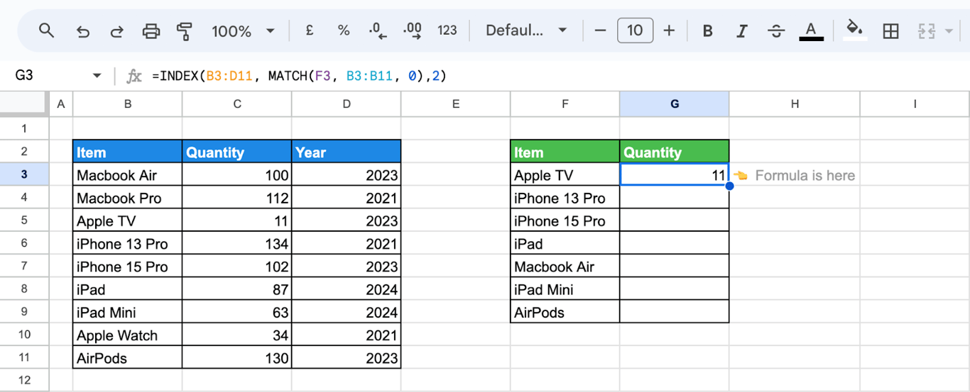
=INDEX(B3:D11, MATCH(F3, B3:B11, 0),2)

The shorter form from the top of this guide gives the same result: point INDEX at the return column only, =INDEX(C3:C11, MATCH(F3, B3:B11, 0)), and the third argument is not needed.

Step 4: Lock the ranges with absolute references

Before copying the formula down, add dollar signs to the ranges. Otherwise each copied row shifts the table down by one, and the last items fall out of it.

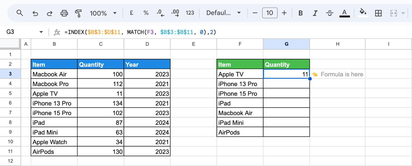
The final formula looks like this:

=INDEX($B$3:$D$11, MATCH(F3, $B$3:$B$11, 0),2)

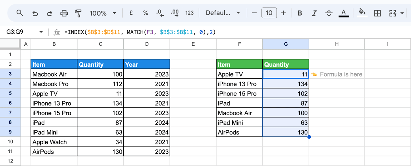
F3 has no dollar signs, so it becomes F4, F5 and so on as the formula is dragged from G3 down.

More ways to use INDEX MATCH

Creating a mini search bar with INDEX and MATCH

A lookup formula that reads its search key from a cell works as a small search box: type an item name in F3 and the result cell shows its quantity.

=INDEX(B3:D11,MATCH(F3,B3:B11,0), 2)

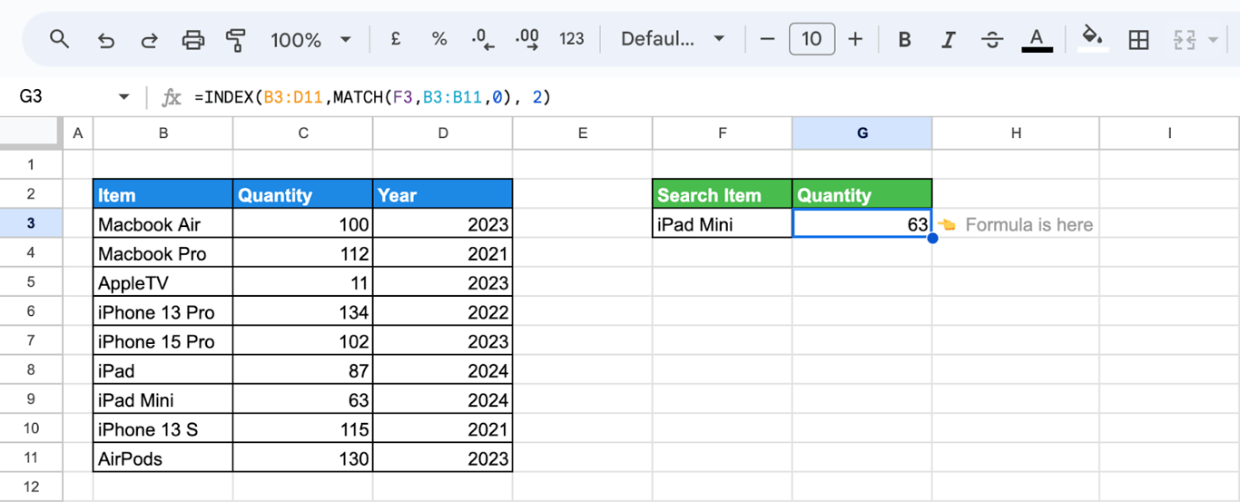
Let’s break it down:

• MATCH(F3,B3:B11,0): The MATCH function searches for a value in column B that matches the input in cell F3.
• INDEX(B3:D11, …, 2): returns the value from the second column of the table in that row.

Wrap the formula in IFERROR to show a message instead of #N/A when the name is not in the list: =IFERROR(INDEX(B3:D11, MATCH(F3, B3:B11, 0), 2), "Not found").

INDEX MATCH with another sheet

To use data on another tab, put the tab name before the range, in single quotes if the name contains spaces, followed by an exclamation mark. Here INDEX returns the quantity from a tab called ‘3. Creating a Mini Search Bar with INDEX and MATCH’, while MATCH searches the item names on the current tab:

=INDEX('3. Creating a Mini Search Bar with INDEX and MATCH'!B3:C11, MATCH(E3, B3:B11, 0), 2)

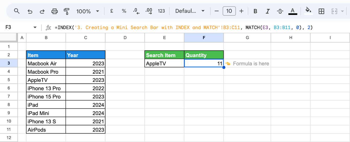
When the names to search are also on the other tab, add the tab name to the MATCH range as well. Both ranges must start on the same row and have the same number of rows, or the result comes from the wrong line.

Multi-criteria searches using INDEX and MATCH

When one column is not enough to identify a row, test several columns at once. To find the quantity of the iPhone 13 Pro produced in 2021, with the item in F3 and the year in G3:

=INDEX(C3:C11, MATCH(1, (F3=B3:B11) * (G3=D3:D11), 0))

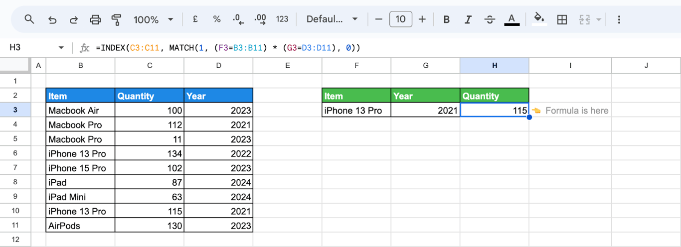
Let’s break down this formula:

• (F3=B3:B11) is TRUE for the rows where the item matches, and (G3=D3:D11) for the rows where the year matches.
• Multiplying them gives 1 only where both are TRUE, and 0 everywhere else. It works as an AND.
• MATCH(1, …, 0) finds the first row with a 1.
• INDEX(C3:C11, …) returns the quantity from that row.

Add a third condition by multiplying with one more comparison.

INDEX MATCH driven by drop-down lists

Typed search keys invite typos. Drop-down lists in the two criteria cells restrict the choice to values that exist.

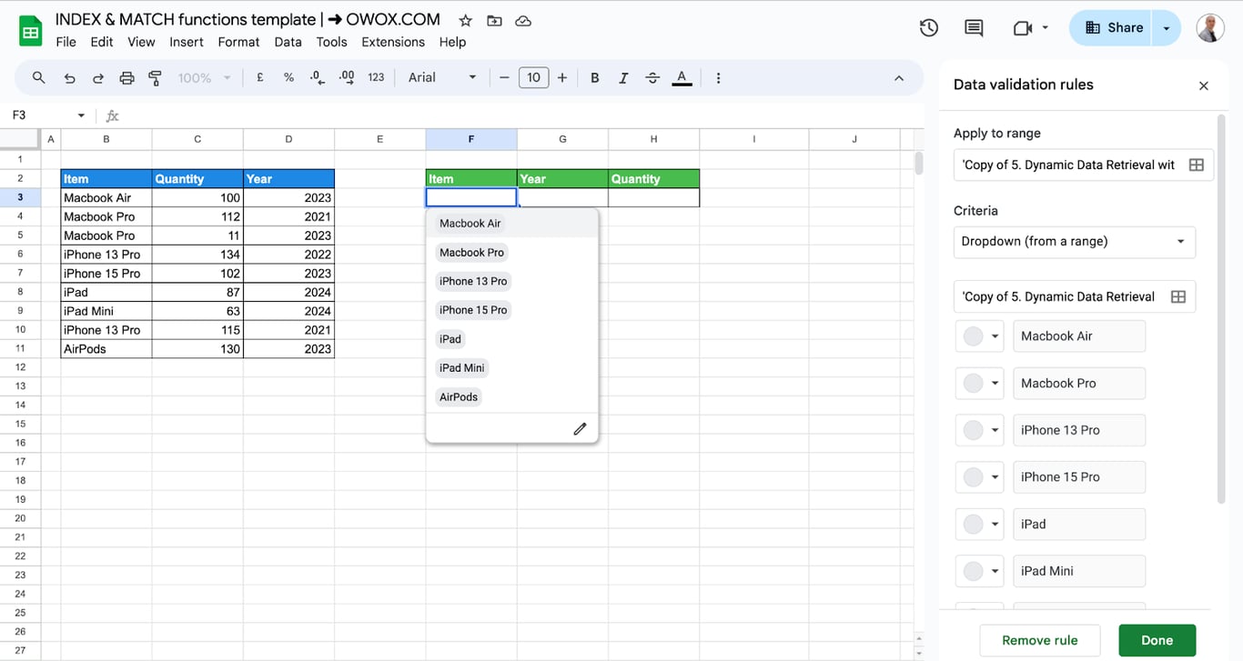
Select cell F3 and go to Data → Data validation.

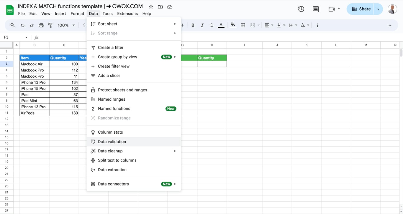
Add a rule, and under Criteria choose Dropdown (from a range).

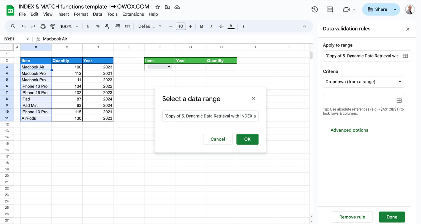
Enter the range with the item names and click Done. Cell F3 now shows an arrow, and clicking it lists the items in your data. Repeat the steps in cell G3 for the years.

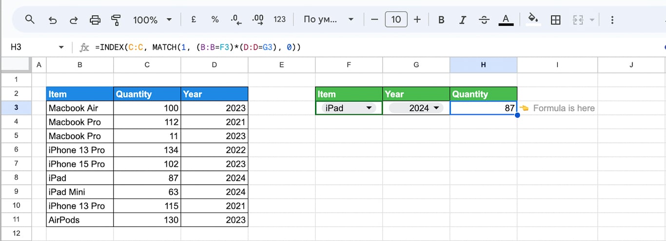
The lookup formula reads both cells:

=INDEX(C:C, MATCH(1, (B:B=F3)*(D:D=G3), 0))

Specifically:

• MATCH(1, (B:B=F3)*(D:D=G3), 0): finds the row where column B equals F3 and column D equals G3.
• INDEX(C:C, …): returns the value of column C in that row.

Whole-column references such as B:B keep working when rows are added. On large sheets they are slower than a bounded range.

Case-sensitive lookup with INDEX, MATCH and EXACT

MATCH and VLOOKUP treat “MacBook Air” and “macbook air” as the same. For a lookup that respects case, compare with EXACT. In this table, used and refurbished items are written in lower case. To return the year of “macbook air”, typed in cell E3:

=INDEX(C3:C11, MATCH(TRUE, ARRAYFORMULA(EXACT(B3:B11, E3)), 0))

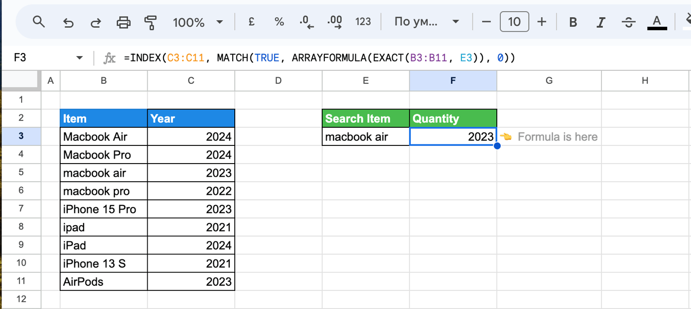
Here’s the breakdown:

• EXACT(B3:B11, E3): creates an array of TRUE and FALSE values, where each element indicates whether the corresponding item in column B exactly matches the search item in E3.
• ARRAYFORMULA(EXACT(B3:B11, E3)): ensures that the EXACT function is applied to the entire range.
• MATCH(TRUE, ARRAYFORMULA(EXACT(B3:B11, E3)), 0): finds the position of the first TRUE in the array, which corresponds to the row where the exact match is found.
• INDEX(C3:C11, …): retrieves the year from the ‘Year’ column corresponding to the matched position.

Why INDEX MATCH returns #N/A or the wrong value

#N/A: the value is not found

⚠️ Error: MATCH returns #N/A when it cannot find the search key, and INDEX passes the error on.

✅ Solution: If the value looks present, compare the two cells exactly. The usual causes are a trailing space, a number stored as text on one side, or a different spelling. TRIM removes extra spaces, and VALUE or TO_TEXT brings both sides to one type.

The wrong row is returned

⚠️ Error: The formula returns a value, but it belongs to another item.

✅ Solution: Check two things. First, the search type: without the 0, MATCH expects sorted data and returns an approximate position. Second, the alignment: the MATCH range and the INDEX range must start on the same row. B3:B11 with C2:C11 returns the value one row too high.

#N/A: the lookup range has several columns

⚠️ Error: MATCH is given a range such as B3:D11.

✅ Solution: MATCH searches one row or one column. Use B3:B11.

#REF!: the position is outside the range

⚠️ Error: INDEX returns #REF! when the row or column number is larger than the range, for example a column number of 4 on a three-column table.

✅ Solution: Make the INDEX range cover every row and column the formula can ask for.

Results change after the formula is copied

⚠️ Error: The first row is right and the rows below are wrong or return #N/A.

✅ Solution: The ranges moved with the formula. Lock them with dollar signs, $B$3:$B$11, as in step 4.

Related Google Sheets functions

Functions that are often used next to INDEX and MATCH, each with its own guide:

• Query Function: Executes complex SQL-like queries within Google Sheets, allowing for detailed data manipulation and retrieval.
• Array Formulas: Enables the performance of multiple calculations over an array of cells, applying a formula to entire columns or rows simultaneously.
• Filter Function: The Filter Function filters out rows in a dataset based on specified conditions, returning only those that meet the specified criteria.
• Pivot Tables: Creates comprehensive summaries from extensive data sets, organizing and comparing distinct values effectively.
• If Function: Evaluates a condition and returns one value if true and another if false, useful for creating conditional formulas.
• ImportRange: Allows data to be imported from one spreadsheet to another, facilitating the sharing and manipulation of data across multiple files.
• Unique Function: Identifies and returns unique rows within a specified data range, eliminating duplicate entries.
• Search Function: Returns the position of a text string within another text string, ignoring case.
• QUERY with UNIQUE: Combines SQL-like filtering with deduplication to return only the distinct rows that match a condition.
• QUERY date filtering: Filters rows by a date or a date range inside a QUERY formula.

A lookup joins two tables, and someone has to own that join

INDEX MATCH is a join done by hand: it attaches a value from one table to a row of another, one cell at a time. It works until the key changes on one side: a product renamed in the CRM, an ID exported as a number in one file and as text in the other, a second row with the same name. The formula then returns #N/A, or worse, the first match of several, and nothing on the sheet says so.

The OWOX Data Marts extension for Google Sheets covers that half. A data analyst publishes a data mart (a table or an SQL query in your data warehouse) and makes it available for reports. In Sheets you open the extension, pick the data mart, tick the columns you want and run it. The rows land in a tab, ready for your formulas.

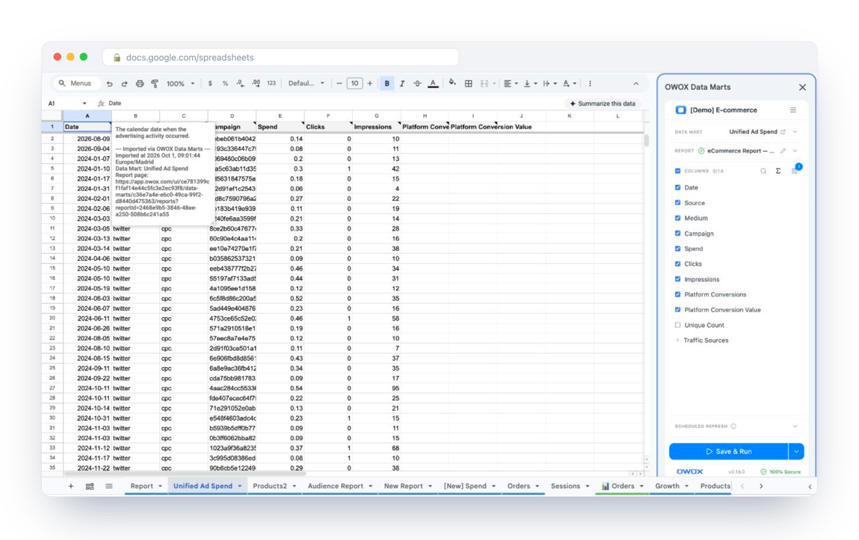
What changes for the person who maintains the sheet:

• Refresh replaces re-export. Refresh current report in the extension menu re-runs the same pull, and a scheduled refresh keeps the tab current without anyone touching it.
• The source is written on the sheet. The header cell of an imported tab carries a note with the data mart it came from, the time of the import and a link to the report.
• No SQL and no warehouse access needed. The analyst decides which data marts and columns are available. You choose from that list.

The extension does not write or change the analyst’s SQL. The join between, say, orders and products is written there once, with a real key, and the columns arrive in the sheet already matched. INDEX MATCH remains the tool for the small lookups that live only in the spreadsheet. The extension comes with the OWOX Cloud plans of OWOX Data Marts; spreadsheet reporting describes both ways data reaches a sheet.

Google Sheets TipsPivot tables in Google Sheets: how to create and use themOctober 2, 2026→Google Sheets TipsQUERY with CONCATENATE in Google Sheets: join two columnsOctober 2, 2026→Google Sheets TipsIF with VLOOKUP in Google Sheets: formulas and examplesOctober 2, 2026→

See all articles →