Retail Data Model: Tables, Keys and Why a Store's Sales Fell
You have been asked why a store's sales fell, and the sales table cannot say. This guide gives the analyst at a multi-store retailer the model that can: ten tables, each with one grain; the two joins that turn a sales figure into a diagnosis; how to split a change into footfall, conversion and basket; four traps measured on a year of demo data (vendor-funded promotions that look like losses, stockouts a sales join cannot see, shrink nobody saw happen, fill rate that hides late deliveries); one definition per metric, a worked example you can run, a free model to start from, and a note to forward to whoever asked.
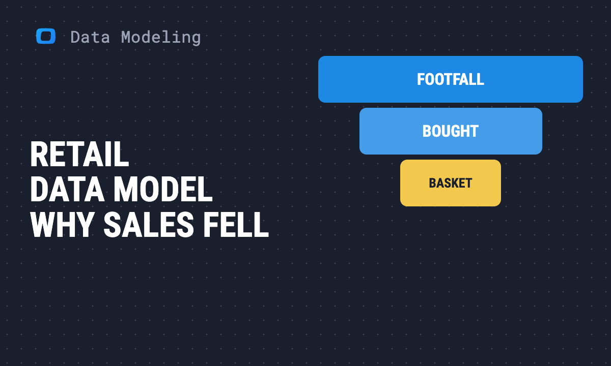
“Sales at San Antonio are down on the quarter. Why?” The sales table can confirm the drop and cannot explain it. To explain it, the sale line, the store’s footfall and the shelf’s closing stock have to share three keys: store, SKU and day. With those joins in place, a weak week splits into four answers that need four different fixes: fewer people came in, fewer of them bought, they spent less per basket, or the line they came for was gone.
This guide is for the analyst at a multi-store retailer who gets that question every Monday. It walks through a ten-table model, the two joins that matter, and four traps we measured on a year of demo data from the free Chain data model. Revenue has accounting rules behind it. Conversion, stockout cost and promotion margin do not, so the definitions are yours to write down, and the last section is a note for whoever asked.
Split the sales change before you explain it
Split the sales change before you explain it
Net sales for a store and period is the product of three numbers:
net sales = footfall × conversion × average basket
Footfall is people through the door, conversion is the share who paid for a basket, and the average basket is net sales per basket. Each one has a different owner. Footfall belongs to marketing, the catchment and the calendar. Conversion belongs to the store floor: queues, availability, staff. The basket belongs to range, price and promotions. A sales report that cannot separate the three sends one question to all of those owners at once.
Here is the split for the six stores of the demo chain, the last 13 weeks against the 13 before. Both windows hold every weekday 13 times, so a Saturday is compared with Saturdays.
| Store (format) | Net sales | Footfall | Conversion | Average basket |
|---|---|---|---|---|
| San Antonio (supermarket) | −2.3% | −1.5% | 0.0% | −0.9% |
| Fort Wayne (neighborhood market) | −2.1% | −1.4% | −0.1% | −0.6% |
| Columbus (supercenter) | −0.5% | +0.2% | −0.2% | −0.5% |
| Chattanooga (neighborhood market) | +0.1% | +0.3% | −0.3% | 0.0% |
| Tucson (supermarket) | +0.9% | +0.5% | +0.4% | −0.1% |
| Reno (neighborhood market) | +1.5% | +2.0% | +0.3% | −0.8% |
Demo data: the synthetic chain behind the Retail Chain model, 13 weeks to 2026-11-01 against 13 weeks to 2026-08-02, run on 2026-11-02. The three levers multiply to the sales change, within rounding.
San Antonio lost people, not buyers. About two thirds of its drop is footfall; the rest is a smaller basket. Its conversion did not move, so the floor is not the first place to look. Reno grew on footfall while its basket shrank almost as fast as San Antonio’s, a fact its sales line hides. The query that produced the table:
WITH p AS (
  SELECT store_id,
    traffic_date > '2026-08-02' AS recent,
    SUM(footfall) AS footfall,
    SUM(transactions) AS baskets,
    SUM(avg_basket_value * transactions) AS sales
  FROM `owox-demo.retail_chain.store_traffic`
  WHERE traffic_date
    BETWEEN '2026-05-04' AND '2026-11-01'
  GROUP BY 1, 2
)
SELECT s.city, s.format,
  ROUND(r.sales / o.sales - 1, 3) AS sales,
  ROUND(r.footfall / o.footfall - 1, 3)
    AS footfall,
  ROUND((r.baskets / r.footfall)
    / (o.baskets / o.footfall) - 1, 3)
    AS conversion,
  ROUND((r.sales / r.baskets)
    / (o.sales / o.baskets) - 1, 3) AS basket
FROM p r
JOIN p o ON o.store_id = r.store_id
  AND r.recent AND NOT o.recent
JOIN `owox-demo.retail_chain.store` s
  ON s.store_id = r.store_id
ORDER BY sales
The split only holds if footfall and sales agree on what a basket is. In the demo data they do: for October, the baskets counted at the door and the distinct basket_id values in the sale lines match to the basket in all six stores. In a real chain the door counter and the tills are two systems, and that reconciliation is the first check to run each month.
The model on one page
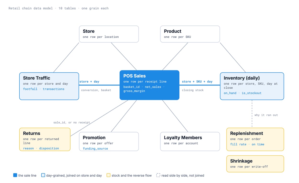
Ten tables. Start each table’s description with its grain, “one row per receipt line”, and make the grain its primary key:
| Table | One row per | Primary key |
|---|---|---|
store |
location | store_id |
product |
SKU | product_id |
promotion |
offer in the promotional calendar | promotion_id |
loyalty_members |
loyalty account | member_id |
pos_sales |
receipt line | sale_id |
store_traffic |
store and day | traffic_id (store, day) |
inventory_daily |
store, SKU and day, at close | snapshot_id (store, SKU, day) |
replenishment |
order to a supplier for one store and SKU | order_id |
shrinkage |
write-off event | shrink_id |
returns |
returned line | return_id |
The two joins that make it a diagnosis
pos_salestostore_trafficon store andsale_date. This is where conversion and the basket come from. The sale line carries a calendar date beside its timestamp for exactly this join: footfall is counted per day, not per second.pos_salestoinventory_dailyon store, product andsale_date. This puts the line’s stock position next to every sale.
The second join has a blind spot: it starts from a sale. A line that sold nothing has no sale row to join from, so the empty shelf, the thing you most want to see, never shows up. Questions about availability start from inventory_daily and join sales onto it. The worked example below shows the difference.
What this model leaves out
Say these limits in the first report, before someone asks a question the tables cannot answer:
- No labour data, so no sales per labour hour or shift cost.
- No distribution centre. Orders run from a store to a supplier.
- No price history beyond promotions, so no price elasticity from a full price ladder.
- No online channel. Traffic is people through a door, not sessions.
- Suppliers are a name on a product and an order, not a table, so a supplier scorecard goes only as far as that name.
OWOX Data Marts
See your first report built in real time. 15 minutes.
- Connect your data warehouse
- Pick your metrics
- Get a live Google Sheets report
In the time it takes to write a ticket. Then imagine never writing that ticket again.
Book a DemoWe'll use your actual use case
Sale lines, baskets and margin
Sale lines, baskets and margin
pos_sales is one row per receipt line, with price, discount, cost and margin on the line. Three rules keep its numbers honest:
- Count baskets, not lines. Transactions are
COUNT(DISTINCT basket_id). They add up across stores and days, because a basket never spans two, and do not add up across categories or promotions, because one basket can hold both. - Margin % is a ratio of sums:
SUM(gross_margin) / SUM(net_sales), at every cut. An average of line margins gives a 50-cent line the same weight as a $50 one. promotion_id IS NULLis full price. The model has no markdown history, so a line is either on an offer or at shelf price.
Vendor-funded promotions look like losses at the till
A promotion has a payer. When the supplier funds the discount, the chain should lose nothing on the line; when the chain funds it, the discount comes out of its margin. The promotion table carries funding_source for that reason. The sale line does not. Here is the demo chain’s year:
| Price type | Net sales | Discount given | Margin at the till | Margin with the vendor’s money added back |
|---|---|---|---|---|
| Full price | $104.4M | $0 | 23.9% | 23.9% |
| Retailer-funded offer | $3.6M | $1.0M | 2.6% | 2.0% |
| Vendor-funded offer | $8.9M | $2.4M | 3.5% | 23.8% |
Demo data, 12 months to 2026-11-01, run on 2026-11-02. The last column is margin plus the vendor-funded discount, over sales at shelf price (net sales plus discount); the retailer-funded row falls because its base is now sales at shelf price.
At the till, vendor-funded offers look nearly as bad as the chain’s own. With the supplier’s money added back they earn what full price earns. In this model, line_cost does not net off the vendor’s money, so gross_margin on a vendor-funded line is the margin before the supplier pays. Read promotions on the last column, or a category manager will cut the deals that cost the chain nothing. Whether your own feed nets the money off depends on how buying books the deal: a discount taken off the supplier’s invoice lowers the cost before it reaches the line, and a claim the supplier pays later does not. Ask buying which kind each deal is.
The retailer-funded offers are where margin goes. In the demo year, app offers and in-store displays funded by the chain sold at a loss on the line, about −6% each. Loyalty-targeted offers kept 17.8% and the weekly circular 11.4%. Whether the losing offers brought extra baskets is a separate question, and it needs the footfall join.
SELECT
  COALESCE(pr.funding_source, 'full price')
    AS price_type,
  ROUND(SUM(s.net_sales)) AS net_sales,
  ROUND(SUM(s.discount)) AS discount,
  ROUND(SUM(s.gross_margin)
    / SUM(s.net_sales), 3) AS till_margin,
  ROUND((SUM(s.gross_margin)
      + SUM(IF(pr.funding_source = 'vendor_funded',
          s.discount, 0)))
    / (SUM(s.net_sales) + SUM(s.discount)), 3)
    AS margin_with_vendor_money
FROM `owox-demo.retail_chain.pos_sales` s
LEFT JOIN `owox-demo.retail_chain.promotion` pr
  USING (promotion_id)
GROUP BY 1
ORDER BY 1
Stock: the sale the sales table never saw
Stock: the sale the sales table never saw
inventory_daily is one row per store, SKU and day, taken at the close of trade: units on hand and their value at cost, units on order, the reorder point, weeks of supply, and is_stockout when the line ended the day with nothing.
“Ended the day empty” is not “was empty all day.” The snapshot is taken once, at close. A line that sold out at 6 pm sold all morning, and a line delivered at 7 am the next day sells again. So the useful question is not “how many stockout days” but “what did the line sell on the day after it closed empty, against the days after it closed stocked.” Here is that comparison for the demo chain, by velocity band:
| Velocity band | Store-SKU-days that closed empty | Average sales the next day, after an empty close | After a stocked close |
|---|---|---|---|
| A (fastest) | 10.7% | $66.45 | $97.04 |
| B | 8.3% | $31.61 | $40.62 |
| C (slowest) | 6.2% | $15.68 | $15.90 |
Demo data, 12 months to 2026-11-01, run on 2026-11-02. Sales per store, SKU and day; days with no sale count as $0.
The fastest lines run out most often, and it costs them about a third of the next day’s sales. A C-band line that closes empty loses almost nothing the next day. Multiplying each band’s gap by its empty-close days gives roughly $3.0M of next-day sales, about 2.5% of the year’s $116.9M. Treat that as a size, not a measurement: the days after an empty close are not otherwise identical to the rest, and some of the spend moves to another line (the worked example shows it).
WITH inv AS (
  SELECT store_id, product_id, snapshot_date,
    is_stockout,
    LAG(is_stockout) OVER (
      PARTITION BY store_id, product_id
      ORDER BY snapshot_date) AS closed_empty
  FROM `owox-demo.retail_chain.inventory_daily`
),
sales AS (
  SELECT store_id, product_id, sale_date,
    SUM(net_sales) AS ns
  FROM `owox-demo.retail_chain.pos_sales`
  GROUP BY 1, 2, 3
)
SELECT p.velocity_band,
  ROUND(AVG(IF(i.is_stockout, 1, 0)), 3)
    AS share_closed_empty,
  ROUND(AVG(IF(i.closed_empty,
    COALESCE(s.ns, 0), NULL)), 2) AS after_empty,
  ROUND(AVG(IF(NOT i.closed_empty,
    COALESCE(s.ns, 0), NULL)), 2) AS after_stocked
FROM inv i
JOIN `owox-demo.retail_chain.product` p
  USING (product_id)
LEFT JOIN sales s
  ON s.store_id = i.store_id
  AND s.product_id = i.product_id
  AND s.sale_date = i.snapshot_date
GROUP BY 1
ORDER BY 1
Why the shelf was empty: fill rate hides late deliveries
An empty shelf has three causes: the store ordered too late, the supplier sent less, or the supplier sent it late. Only replenishment, one row per order, separates them. It carries ordered and received quantities, the promised and actual dates, and two service measures: fill_rate_pct, the share of the order that arrived, and is_on_time.
In the demo chain the average fill rate on completed orders is 96.7%, which reads as a supplier base that delivers. Only 79.4% of received orders arrived both on time and in full. One order in five missed on one count or the other, and a punctual short shipment is still an empty shelf. Report on-time-in-full, and keep the two halves beside it so buying knows which half to raise with the supplier. Two scale traps on the way: fill_rate_pct runs from 0 to 100, not 0 to 1, and open orders have no received_at, so leave them out of lead time instead of counting them as received today.
Shrink and returns: the reverse flow
Shrink and returns: the reverse flow
Shrink is stock the chain paid for and never sold. shrinkage holds one row per write-off with its reason (theft, damage, expiry, admin error) and, as important, how it was found. A loss caught at the receiving door, by security or by a self-checkout audit has its cause attached. A loss found at a cycle count, when the book and the shelf disagree, does not: it is unknown shrink, and by then the cause is gone. Each loss is valued twice, at cost for margin questions and at shelf price for shrink as a percentage of sales.
In the demo chain, shrink at shelf price ran from 1.9% of net sales (the Columbus supercenter) to 2.6% (the Fort Wayne neighborhood market), and 52% to 55% of it in every store surfaced only at a cycle count. More than half of the loss had no cause attached when it was found.
Self-checkout is the comparison people reach for next, and the model is explicit that it is a side-by-side read, not a join: sum checkout_type = 'self_checkout' sales per store, and set that share beside the store’s shrink found by self-checkout audits. In the demo chain, Columbus has the highest self-checkout share of trade (28.7%) and the lowest shrink. A single store pair proves nothing either way; the read needs months and formats held constant.
Returns cost twice: the refund, and the value lost when the returned unit cannot go back on the shelf at full price. returns carries the reason (damaged, defective, wrong item, changed mind, expired, price dispute) and the disposition (resell, markdown, back to the vendor, disposal). It also carries store and product directly, because a return without a receipt has no sale_id and so no sale line to take them from. In the demo chain refunds were 2.7% to 3.2% of net sales, and 15% to 22% of returned lines, depending on the store, came back without a receipt.
Compare stores within a format
Compare stores within a format
store holds format, selling area, region and opening date, and the format comes first. In October the demo supercenter in Columbus took $4.38M, more than twice any other store, at $24 per square foot of selling area. The three neighborhood markets took $0.91M to $0.94M each at $58 to $65 per square foot. Ranked across formats, the biggest store is the least productive; ranked within its format, it has no peer at all. Hold format constant, and compare like for like only after a store has 13 months behind it: the demo chain’s newest store opened on 2026-04-06, so it has no last year to compare with until May 2027.
The loyalty table answers a different question: who. In the demo chain 65% of net sales was rung on an identified loyalty basket. Per-member figures, such as spend per member or visits per member, are taken over that identified part only, and the anonymous 35% still counts toward the store’s trade.
One definition per metric
Revenue has an accounting standard behind it. Conversion, promotion margin and stockout rate do not, so whoever writes the definition owns the number. Write them down once. Defensible defaults:
| Metric | Definition | Reads |
|---|---|---|
| Net sales | Sum of line net_sales after discount |
pos_sales |
| Transactions | Distinct baskets | pos_sales |
| Conversion rate | Transactions ÷ footfall, both summed at the report’s grain; never an average of daily rates | store_traffic |
| Average basket | Net sales ÷ transactions | pos_sales or store_traffic |
| Sales per visitor | Net sales ÷ footfall (conversion × average basket) | store_traffic |
| Gross margin % | Sum of margin ÷ sum of net sales | pos_sales |
| Promotion margin | Margin plus vendor-funded discount, over sales at shelf price | pos_sales, promotion |
| Stockout rate | Store-SKU-days that closed empty ÷ all store-SKU-days, by velocity band | inventory_daily, product |
| On-time-in-full | Received orders that arrived by the promised date and in full ÷ received orders; open orders excluded | replenishment |
| Shrink % | Shrink at shelf price ÷ net sales; known and unknown shown apart | shrinkage, pos_sales |
| Sales per square foot | Net sales ÷ selling area, within one format | pos_sales, store |
| Loyalty sales share | Net sales on identified baskets ÷ net sales | pos_sales |
Three choices move numbers most:
- Conversion’s grain. An average of daily conversion rates weights a quiet Tuesday like a busy Saturday. In the demo chain the two happen to agree to a tenth of a point because conversion barely varies; in a chain where it does vary, they will not.
- Whose money a promotion spent. The same offer is a loss or break-even depending on the payer. Decide with buying how vendor money is booked before anyone ranks promotions.
- What a stockout is. A closing snapshot says the line ended empty, not how long it was empty. If your stock system can give intraday positions, that is a better definition, and a different table.
A worked example you can run
One store, two Mondays a week apart, ten visitors each day. Literal rows, so the first query runs in any BigQuery project as written, and the second runs once you paste the first one’s pos_sales rows into it. Milk is $4, coffee $12, a towel $6. On the second Monday the coffee had closed empty the night before.
The first query splits each day into the three levers:
WITH store_traffic AS (
  SELECT * FROM UNNEST([
    STRUCT('S1' AS store_id,
      DATE '2026-03-02' AS traffic_date,
      10 AS footfall),
    ('S1', DATE '2026-03-09', 10)
  ])
),
pos_sales AS (
  SELECT * FROM UNNEST([
    STRUCT('S1' AS store_id,
      DATE '2026-03-02' AS sale_date,
      'B1' AS basket_id,
      'MILK' AS product_id,
      2 AS quantity,
      8.00 AS net_sales),
    ('S1', '2026-03-02', 'B1', 'COFFEE', 1, 12.00),
    ('S1', '2026-03-02', 'B2', 'COFFEE', 1, 12.00),
    ('S1', '2026-03-02', 'B3', 'MILK', 1, 4.00),
    ('S1', '2026-03-02', 'B4', 'COFFEE', 2, 24.00),
    ('S1', '2026-03-02', 'B5', 'MILK', 1, 4.00),
    ('S1', '2026-03-02', 'B5', 'TOWEL', 1, 6.00),
    ('S1', '2026-03-02', 'B6', 'COFFEE', 1, 12.00),
    ('S1', '2026-03-02', 'B7', 'MILK', 2, 8.00),
    ('S1', '2026-03-02', 'B8', 'TOWEL', 1, 6.00),
    ('S1', '2026-03-09', 'C1', 'MILK', 2, 8.00),
    ('S1', '2026-03-09', 'C2', 'MILK', 1, 4.00),
    ('S1', '2026-03-09', 'C3', 'TOWEL', 1, 6.00),
    ('S1', '2026-03-09', 'C4', 'MILK', 2, 8.00),
    ('S1', '2026-03-09', 'C5', 'MILK', 1, 4.00),
    ('S1', '2026-03-09', 'C5', 'TOWEL', 1, 6.00),
    ('S1', '2026-03-09', 'C6', 'TOWEL', 1, 6.00),
    ('S1', '2026-03-09', 'C7', 'MILK', 2, 8.00),
    ('S1', '2026-03-09', 'C8', 'TOWEL', 1, 6.00)
  ])
),
day AS (
  SELECT t.traffic_date,
    t.footfall,
    COUNT(DISTINCT s.basket_id) AS transactions,
    SUM(s.net_sales) AS net_sales
  FROM store_traffic t
  JOIN pos_sales s
    ON s.store_id = t.store_id
    AND s.sale_date = t.traffic_date
  GROUP BY 1, 2
)
SELECT traffic_date,
  footfall,
  transactions,
  ROUND(transactions / footfall, 2) AS conversion,
  ROUND(net_sales / transactions, 2) AS avg_basket,
  net_sales
FROM day
ORDER BY traffic_date| Day | Footfall | Transactions | Conversion | Average basket | Net sales |
|---|---|---|---|---|---|
| 2026-03-02 | 10 | 8 | 0.8 | $12.00 | $96 |
| 2026-03-09 | 10 | 8 | 0.8 | $7.00 | $56 |
Sales fell 42% with the same visitors and the same buyers. Every dollar of the drop is in the basket. A report that stopped here would send the question to pricing.
The second query starts from the stock position the night before, keeps the pos_sales rows from the first query, and joins sales onto it:
WITH inventory_daily AS (
  SELECT * FROM UNNEST([
    STRUCT('S1' AS store_id,
      'MILK' AS product_id,
      DATE '2026-03-08' AS snapshot_date,
      40 AS on_hand_units,
      FALSE AS is_stockout),
    ('S1', 'COFFEE', '2026-03-08', 0, TRUE),
    ('S1', 'TOWEL', '2026-03-08', 25, FALSE)
  ])
),
pos_sales AS (
  -- the same 19 rows as in the first query
)
-- Start from the stock position, not from the sales:
-- a line that sold nothing has no sale row to join from.
SELECT i.product_id,
  i.is_stockout AS empty_at_last_close,
  SUM(IF(s.sale_date = '2026-03-02',
    s.net_sales, 0)) AS sales_last_week,
  SUM(IF(s.sale_date = '2026-03-09',
    s.net_sales, 0)) AS sales_today
FROM inventory_daily i
LEFT JOIN pos_sales s
  ON s.store_id = i.store_id
  AND s.product_id = i.product_id
GROUP BY 1, 2
ORDER BY 1| Product | Empty at last close | Sales last Monday | Sales this Monday |
|---|---|---|---|
| COFFEE | true | $60 | $0 |
| MILK | false | $24 | $32 |
| TOWEL | false | $12 | $24 |
The basket shrank because the coffee was gone. Coffee took $60 the Monday before and nothing this Monday. Shoppers spent $20 more on milk and towels, so the store lost $40, not $60. Join the other way, from the sale lines to the stock, and coffee never appears, because there is no coffee line to join from.
Start from a free model
OWOX publishes a free Chain data model: 10 Data Marts for a US general-merchandise-and-grocery chain, the same ten tables as above, with the joins on store, SKU and day already declared and the metrics in this article defined as calculated fields (Transactions, Average Transaction Value, Gross Margin %, Conversion Rate, Sales per Visitor, Loyalty Sales Share). It opens on OWOX Model Canvas, where you can edit it and export it as an OKF bundle, one Markdown file per table; the definition is on GitHub.
Adapt three things before you load your own data:
- Add the vendor’s money. Promotion margin as defined above needs the vendor-funded amount on the line, or a funding amount per promotion.
- Add what the model leaves out where you have it: labour hours for sales per labour hour, a distribution centre between store and supplier, an online channel.
- Decide the stockout definition if your stock system can do better than a closing snapshot.
It describes the business; it does not connect to your POS or stock system. For the design ideas behind it, see star schema and the three types of fact tables: pos_sales is a transaction fact, inventory_daily a periodic snapshot. Other models in this series include the e-commerce data model for an online store and the clinic network data model.
Where OWOX Data Marts fits, and what it does not do
Where OWOX Data Marts fits, and what it does not do
Everything above is warehouse SQL that any BI tool can read. It is written in BigQuery’s dialect and ports to Snowflake, AWS Redshift, AWS Athena or Databricks with small changes. OWOX Data Marts takes on three parts:
- Getting the data in: a POS or stock system’s API can be added as a custom connector, described in a configuration file; the built-in cover the ad platforms.
- Owning the definitions: each table becomes a Data Mart with its grain and primary key, together forming the Model, and each metric is defined once as a calculated field. quality checks on primary key uniqueness catch a till export loaded twice.
- Delivery: reports to Sheets on a schedule; through OWOX MCP for Claude and ChatGPT, part of OWOX Data Marts Cloud, either assistant can query the published Data Marts, and the rows returned are sent to that AI provider. A question such as “why did San Antonio’s sales fall last quarter?” then runs on the joins the analyst declared, not on the assistant’s guess at which tables belong together.
What it does not do: it does not count people at the door, it does not decide whether a vendor-funded discount is the chain’s cost, and it does not replace finance’s figures. Those are the business’s decisions; the model makes them visible.
For the person who asked
A note from the analyst to whoever asked why sales fell, ready to forward:
- I can split every store’s sales change into footfall, conversion and average basket, every week, and show which lines closed the previous day empty.
- Sales alone cannot say why. In our demo chain, San Antonio’s 2.3% fall last quarter was mostly fewer visitors (−1.5%) and a smaller basket (−0.9%); the share of visitors who bought did not change. That points at the catchment and the range, not at the store floor.
- An empty shelf does not show up in a sales report, because nothing was sold. I will report availability from the stock position, by velocity band, starting with the fastest-selling lines.
- Some promotions look like losses because the supplier’s share is not in the margin. I will report promotion margin with the vendor’s money added back, once buying confirms which deals are vendor-funded and how that money is booked.
- Decisions for you:
- Is a line “out of stock” when it closes the day empty, or do we need intraday stock?
- Are promotions judged on margin or on sales, and with the vendor’s money counted?
- Which formats are compared with each other, and from how many months after opening is a store like-for-like?
- Is shrink reported at cost or at shelf price, and do we show unknown shrink separately?
- Until you decide, I will treat a closing-empty day as a stockout day, report promotion margin both ways, compare stores only within their format and after 13 months of trade, report shrink at shelf price with unknown shrink apart, and say so at the top of the report.
Turn your data into decisions.
Governed data marts give you the clean foundation ML needs to actually work.
- No AI hallucinations
- Analyst-governed definitions
- Every number traces to SQL