ROUND, CEILING and FLOOR in Google Sheets: which rounding function to use
ROUND rounds to a number of decimal places, CEILING and FLOOR round up or down to a multiple, and MROUND rounds to the nearest multiple. This guide compares all the rounding functions of Google Sheets on the same numbers, shows how to round to the nearest 0.5, 5 or 10 and to quarter hours, and explains what each function does with negative numbers.

Google Sheets rounds in two ways. ROUND, ROUNDUP and ROUNDDOWN round to a number of decimal places. CEILING, FLOOR and MROUND round to a multiple of a number you choose, such as 0.5, 5 or 10.
=ROUND(87.16, 0)
=CEILING(87.16, 10)
=FLOOR(87.16, 10)
The results are 87, 90 and 80.
Which rounding function to use
Which rounding function to use
| To round | Use | 4.3 becomes | -4.3 becomes |
|---|---|---|---|
| To the nearest whole number or decimal place | ROUND(value, places) |
4 | -4 |
| Always away from zero | ROUNDUP(value, places) |
5 | -5 |
| Always toward zero | ROUNDDOWN(value, places) |
4 | -4 |
| Up to a multiple | CEILING(value, factor) |
5 | -4 |
| Down to a multiple | FLOOR(value, factor) |
4 | -5 |
| To the nearest multiple | MROUND(value, factor) |
4 | see below |
| Down to a whole number | INT(value) |
4 | -5 |
| Cut off the decimals | TRUNC(value) |
4 | -4 |
The quick answers to the common tasks:
| Task | Formula | 7.3 becomes |
|---|---|---|
| Round to the nearest 0.5 | =MROUND(A2, 0.5) |
7.5 |
| Round up to the next 0.5 | =CEILING(A2, 0.5) |
7.5 |
| Round down to the previous 0.5 | =FLOOR(A2, 0.5) |
7 |
| Round to two decimal places | =ROUND(A2, 2) |
7.3 |
| Round to the nearest 10 | =ROUND(A2, -1) |
10 |
| Round up to the next 5 | =CEILING(A2, 5) |
10 |
ROUND, ROUNDUP and ROUNDDOWN
=ROUND(value, [places])
- value: the number to round.
- places: the number of decimal places. Optional, 0 by default. A negative number rounds to the left of the decimal point: -1 to tens, -2 to hundreds.
ROUNDUP and ROUNDDOWN take the same arguments.
=ROUND(C3, 0)
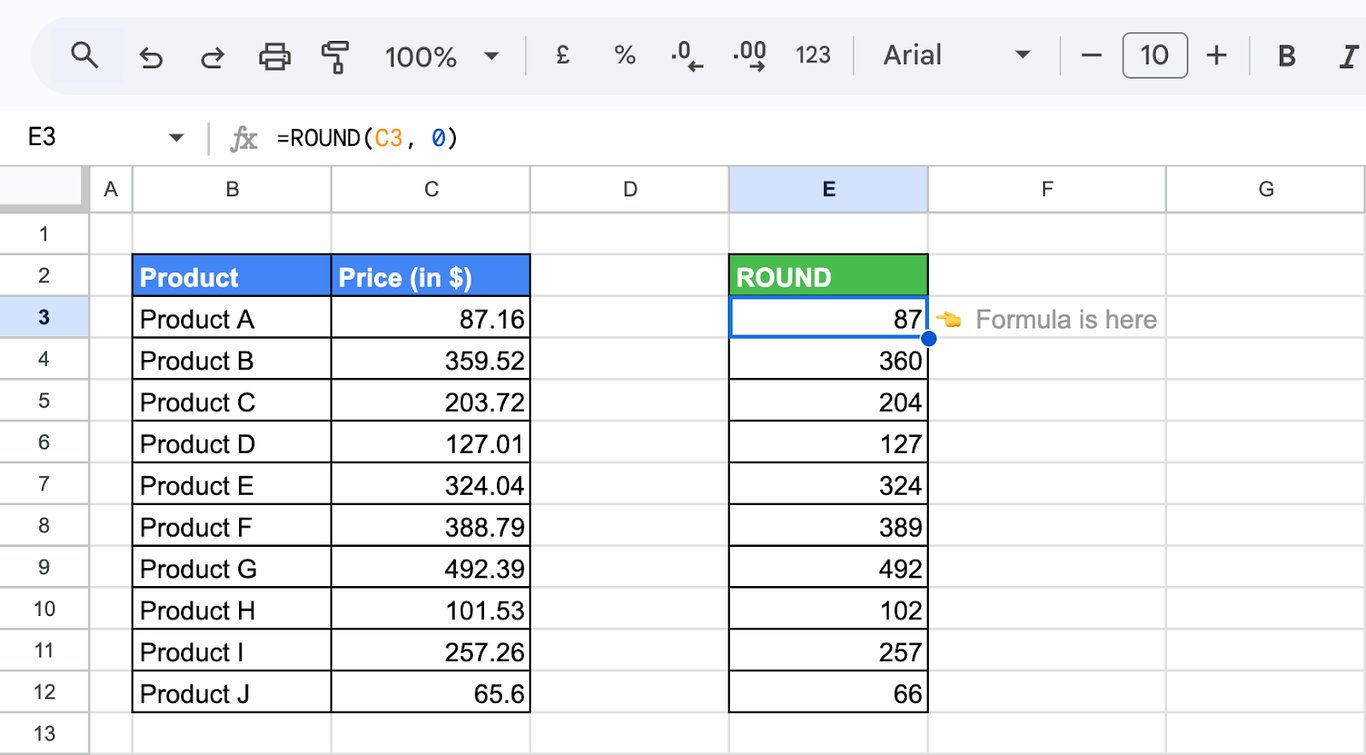
ROUND goes to the nearest value, and a 5 rounds away from zero: 2.5 becomes 3 and -4.5 becomes -5.
=ROUNDUP(C3)
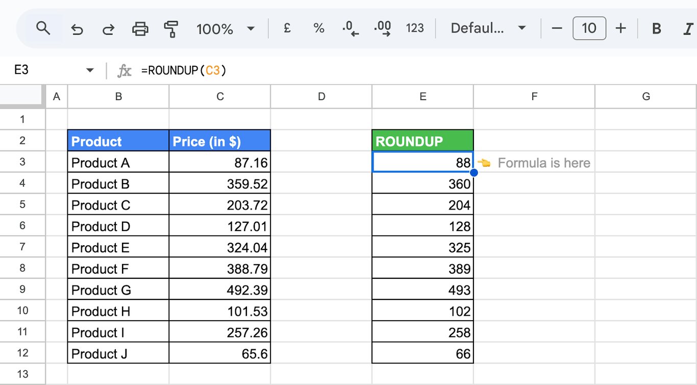
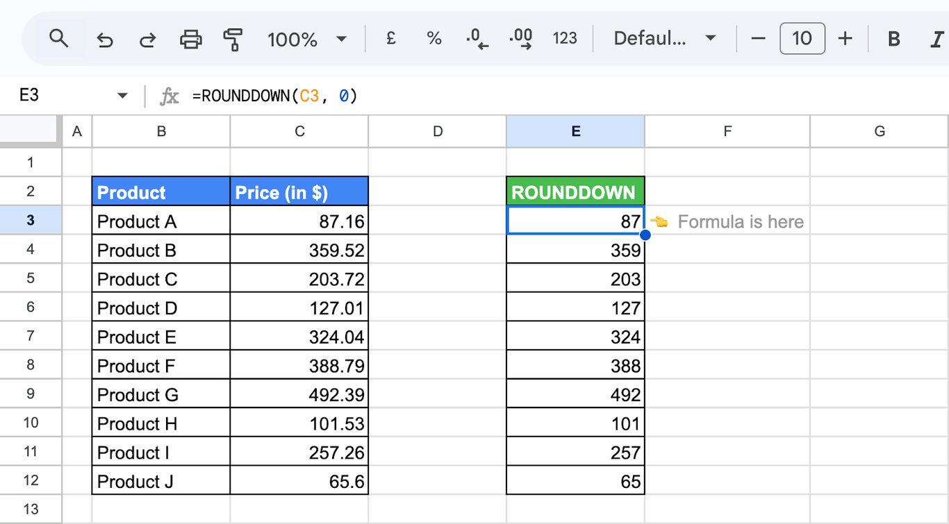
=ROUNDDOWN(C3, 0)
Round to tens, hundreds or thousands
=ROUND(C3, -1)
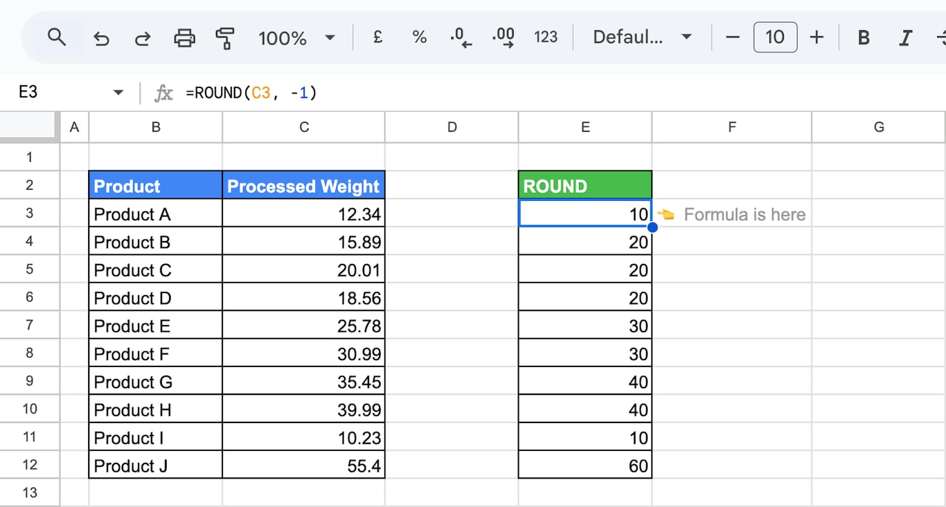
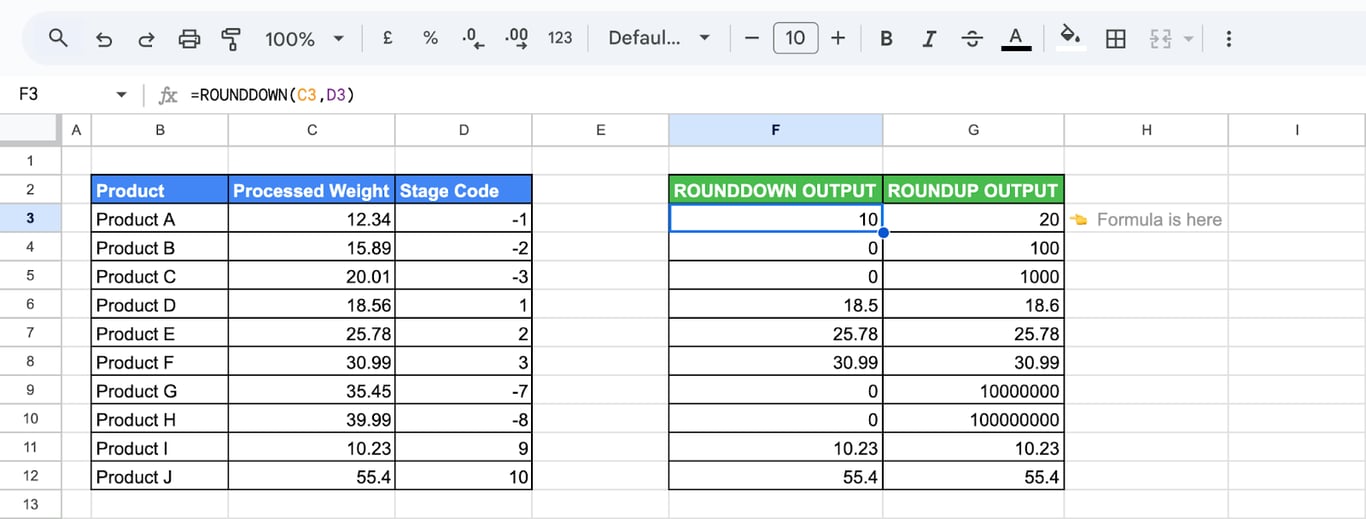
=ROUND(1234.567, -2) returns 1200. The places can come from a cell, which lets one formula round different rows to different precision:
=ROUNDDOWN(C3, D3)
Negative numbers
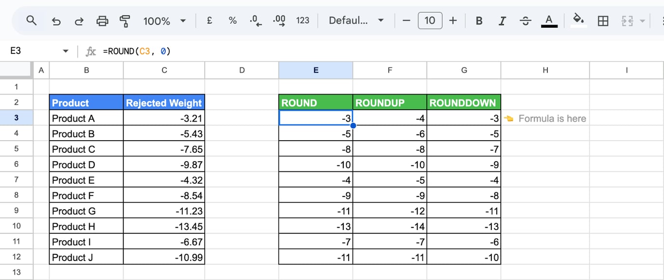
“Up” in ROUNDUP means away from zero, and “down” in ROUNDDOWN means toward zero:
Remove the time from a date
A date with a time is a number with decimals: the whole part is the day, the fraction the time. Rounding down leaves the date:
=ROUNDDOWN(C3, 0)
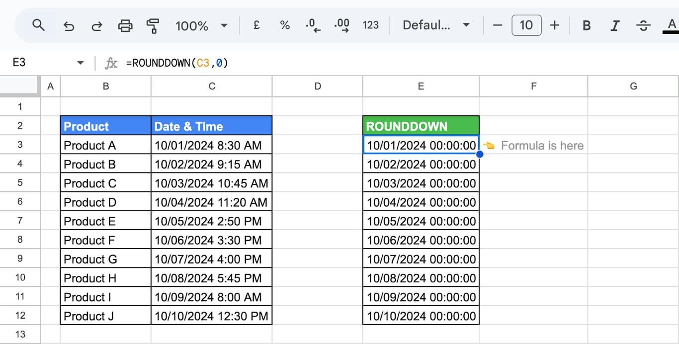
INT(C3) does the same. Format the result as a date to hide the zero time. See dates and times.
ROUND or a number format
The decimal buttons on the toolbar change how a number looks, not the number. A cell that shows 0.3 may hold 0.33333, and a sum of such cells adds the full values, so a column of rounded-looking numbers can add up to a total that seems off by a cent. ROUND changes the value itself. Use the format for display and ROUND when the rounded number goes into further calculations, such as invoice lines.
OWOX Data Marts
See your first report built in real time. 15 minutes.
- Connect your data warehouse
- Pick your metrics
- Get a live Google Sheets report
In the time it takes to write a ticket. Then imagine never writing that ticket again.
Book a DemoWe'll use your actual use case
CEILING and FLOOR: round to a multiple
CEILING and FLOOR: round to a multiple
=CEILING(value, [factor])
=FLOOR(value, [factor])
- value: the number to round.
- factor: the multiple to round to. Optional, 1 by default.
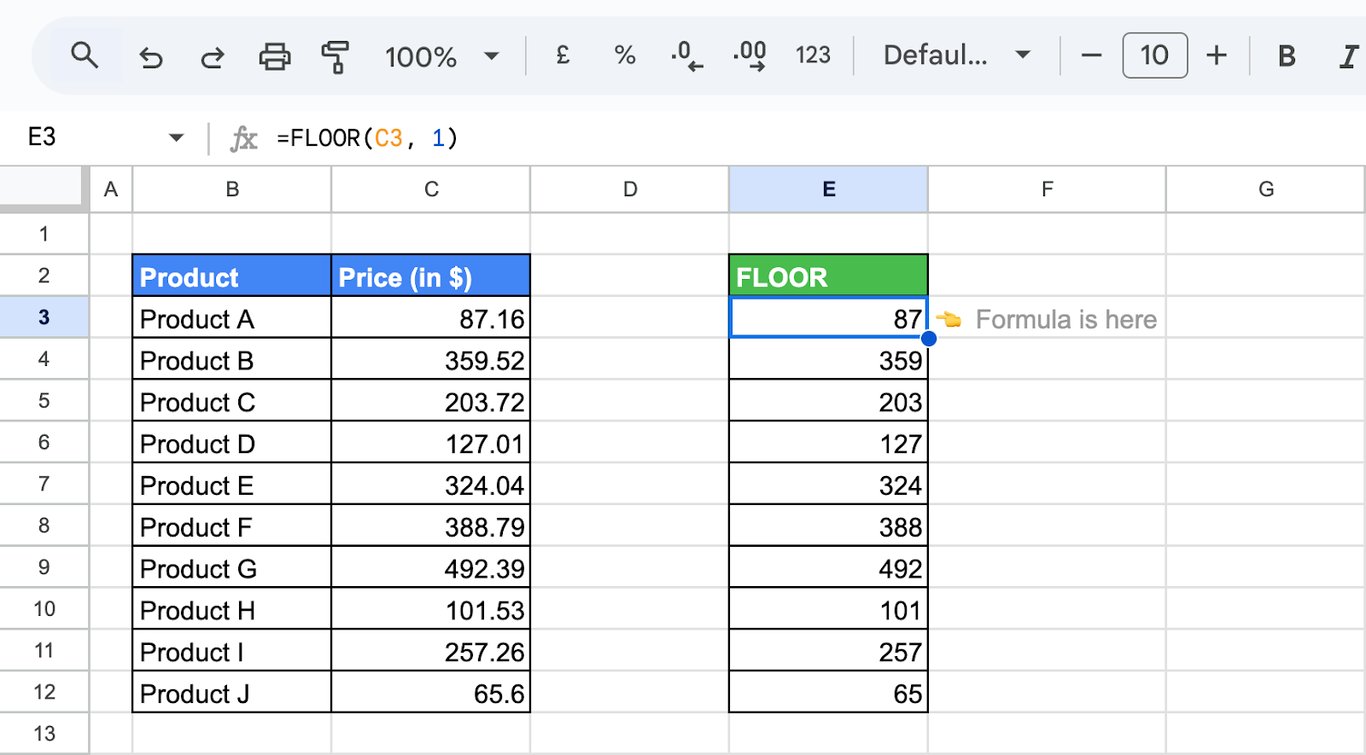
CEILING goes up to the next multiple, FLOOR down to the previous one.
=CEILING(C3, 1)
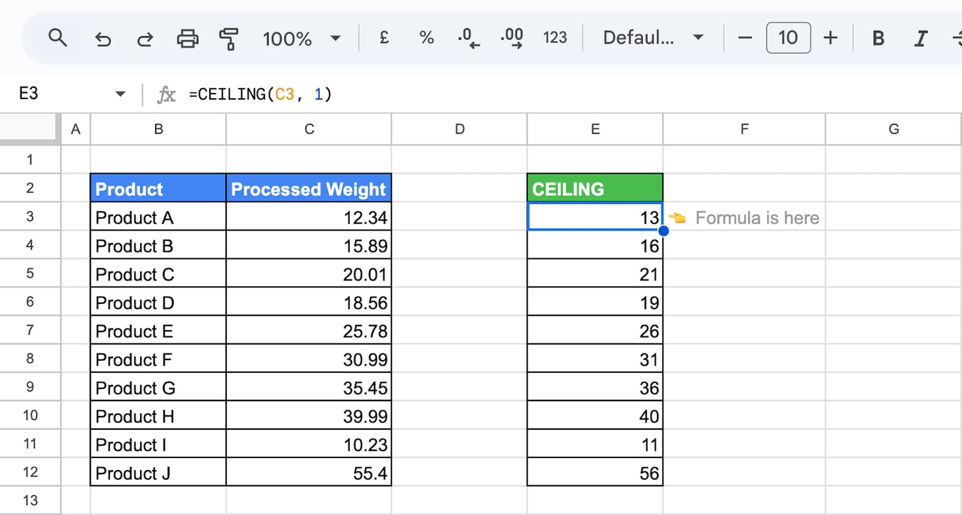
=FLOOR(C3, 1)
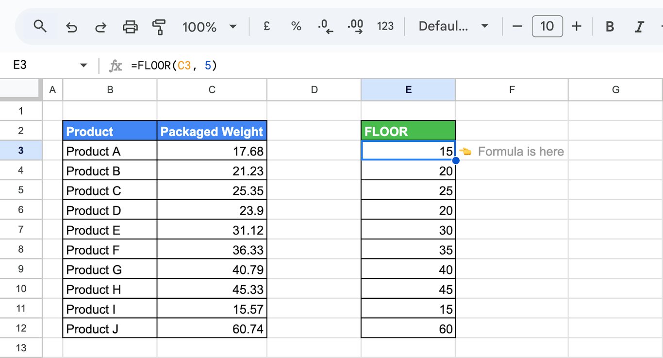
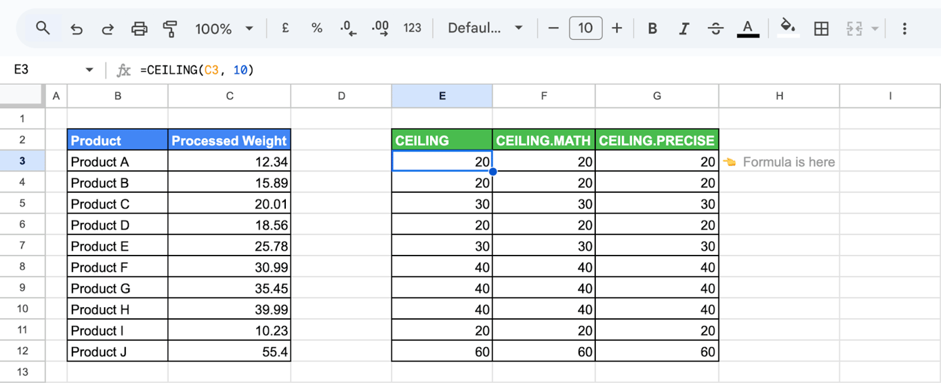
To the nearest 5 or 10
=FLOOR(C3, 5)
=CEILING(C3, 10)
To the nearest 0.5
=CEILING(C3, 0.5)
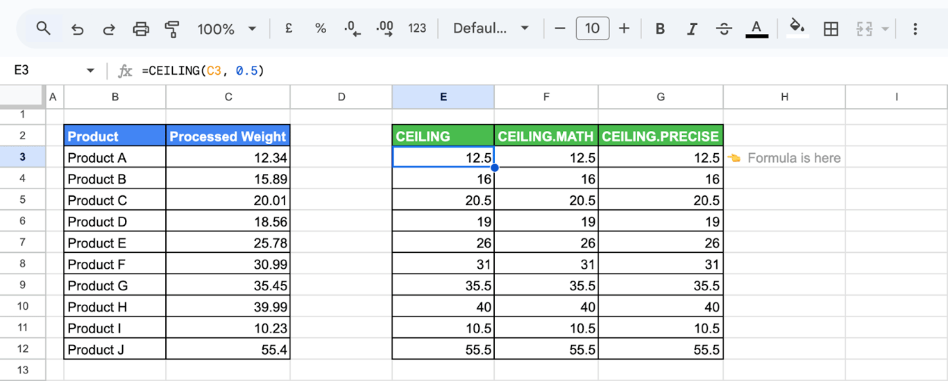
CEILING always goes up and FLOOR always down. To round to the nearest half, use MROUND:
=MROUND(C3, 0.5)
MROUND returns 12.5 for 12.34 and 16 for 15.89, but 12 for 12.2, where CEILING would return 12.5. The same works for any step: =MROUND(A2, 5), =MROUND(A2, 0.25).
A factor from a cell
=CEILING(C3, D3)
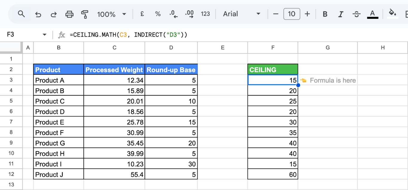
Each row is rounded up to a multiple of its own base. The formula in the screenshot reads the base through INDIRECT, which is not needed: a plain reference to D3 gives the same result and follows the row when the formula is copied down.
CEILING.MATH, CEILING.PRECISE, FLOOR.MATH, FLOOR.PRECISE
CEILING.MATH, CEILING.PRECISE, FLOOR.MATH, FLOOR.PRECISE
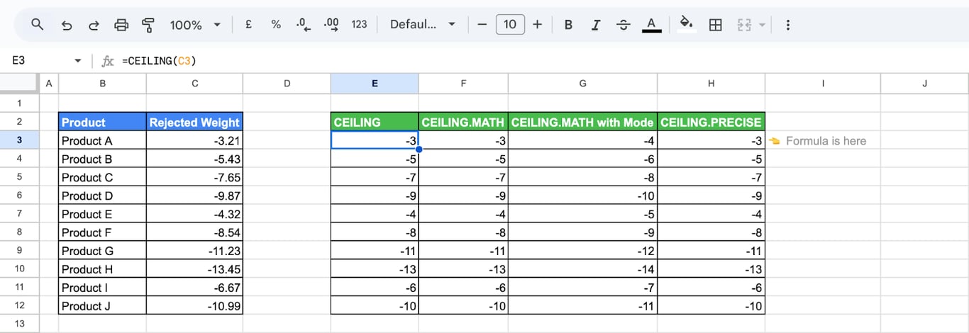
These four mirror the Excel functions of the same names. For positive numbers they return the same as CEILING and FLOOR. They differ in how they treat negative numbers:
=CEILING.MATH(number, [significance], [mode])
=FLOOR.MATH(number, [significance], [mode])
=CEILING.PRECISE(number, [significance])
=FLOOR.PRECISE(number, [significance])
| Formula | Result for -4.3 | Direction |
|---|---|---|
=CEILING(-4.3) |
-4 | Toward zero |
=CEILING(-4.3, -1) |
-5 | Away from zero |
=CEILING.MATH(-4.3) |
-4 | Toward zero |
=CEILING.MATH(-4.3, 1, -1) |
-5 | Away from zero (mode set) |
=CEILING.PRECISE(-4.3) |
-4 | Toward zero |
=FLOOR(-4.3, 1) |
-5 | Away from zero |
=FLOOR(-4.3, -1) |
-4 | Toward zero |
=FLOOR.MATH(-4.3) |
-5 | Away from zero |
=FLOOR.MATH(-4.3, 1, 1) |
-4 | Toward zero (mode set) |
=FLOOR.PRECISE(-4.3) |
-5 | Away from zero |
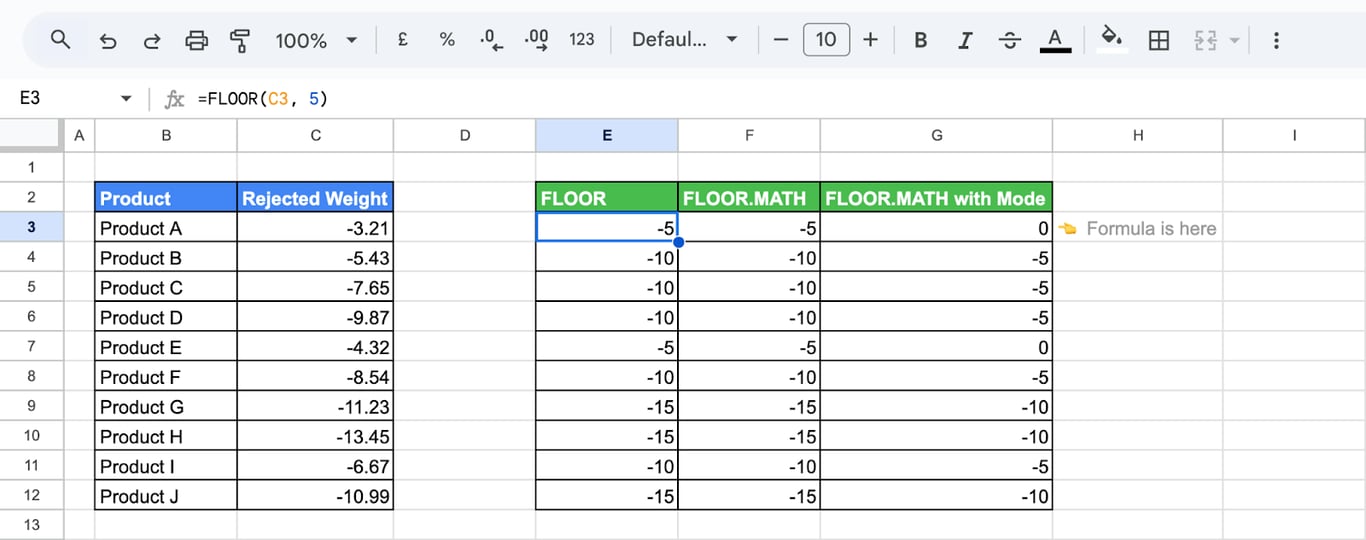
“Up” for the ceiling functions means toward positive infinity, so -4.3 goes to -4. The mode argument of the .MATH functions, when it is not zero, reverses the direction for negative numbers.
Round time
Time is a fraction of a day, so it rounds to a multiple like any number. Give the step as a time:
=FLOOR(A2, "0:30")rounds 9:47 down to 9:30.=CEILING(A2, "0:15")rounds 9:47 up to 10:00.=MROUND(A2, "0:15")rounds 9:47 to the nearest quarter, 9:45.
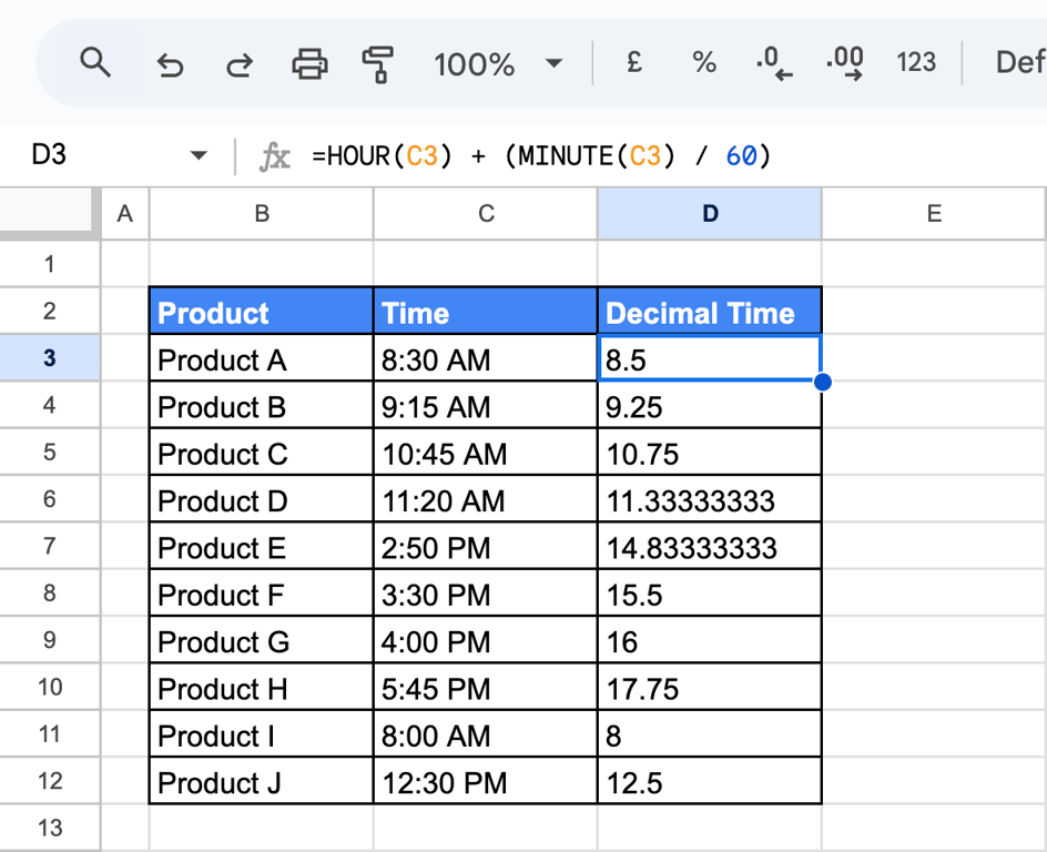
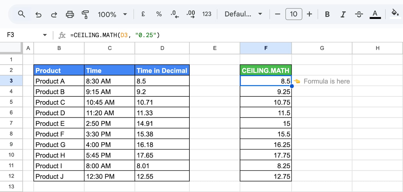
Format the result as a time. If the hours are kept as decimal numbers, as on a timesheet, the step is a decimal too. This formula turns a time into decimal hours:
=HOUR(C3) + (MINUTE(C3) / 60)
=CEILING.MATH(D3, 0.25)
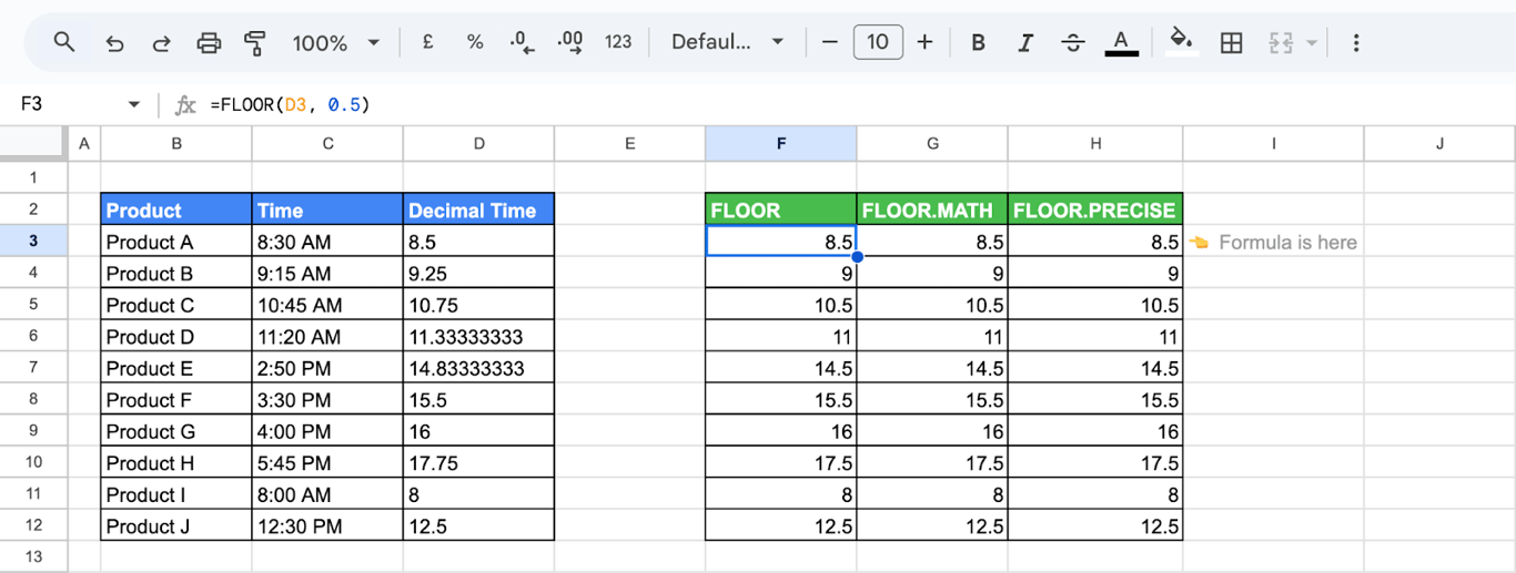
=FLOOR(D3, 0.5)
Rounding inside other formulas
Rounding inside other formulas
Round the result of a calculation, not its inputs: wrap the whole formula.
=CEILING(SUM(C3:D3), 1)
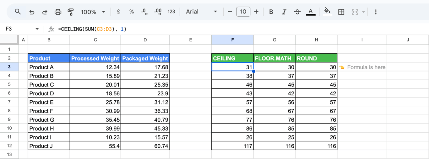
The factor must not be 0: =CEILING(SUM(C3:D3), 0) returns 0, and FLOOR with a factor of 0 returns #DIV/0!.
=ROUND(AVERAGE(C3:C12), 1)
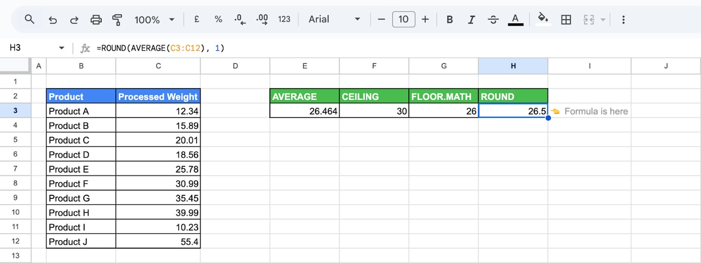
With IF, the precision can depend on the value:
=IF(C3 < 30, ROUND(C3, 0), ROUND(C3, 1))
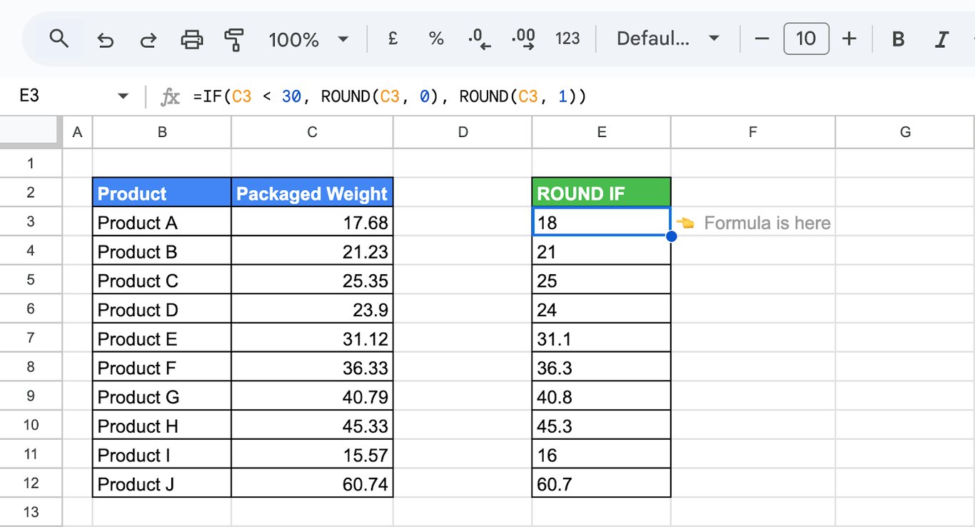
Rounding each row and then adding gives a different total from adding first and rounding once. Decide which one the report needs, and use the same order everywhere.
Errors and wrong results
⚠️ Error: #NUM!
✅ Solution: The value is positive and the factor negative, as in =CEILING(4.3, -1), or MROUND was given a value and a factor of different signs. Use the same sign for both.
⚠️ Error: #DIV/0!
✅ Solution: FLOOR or MROUND has a factor of 0. Often the factor comes from an empty cell.
⚠️ Error: CEILING returns 0.
✅ Solution: The factor is 0. Set it to 1 for whole numbers.
⚠️ Error: #VALUE!
✅ Solution: The value is text, such as “abc” or a number with a currency sign typed as text. Convert it with VALUE first.
⚠️ Error: A total does not match the sum of the rounded numbers on screen.
✅ Solution: The cells are formatted to fewer decimals but hold the full values. Round with ROUND where the rounded value matters.
⚠️ Error: A negative number rounds the “wrong” way.
✅ Solution: Check the table above: CEILING and INT move toward positive and negative infinity, ROUNDUP and ROUNDDOWN away from and toward zero.
Related Google Sheets functions
Related Google Sheets functions
- SUM functions: SUM, SUMIF and SUMIFS.
- AVERAGE functions: The mean, with and without conditions.
- MAX, MIN and MEDIAN: The largest, smallest and middle values.
- TEXT: Show a number with a fixed number of decimals inside a text.
- IF: Round differently depending on a condition.
- Dates and times: Why time rounds like a number.
- PERCENTILE and QUARTILE: Cut points of a distribution.
Rounding is the last step, the numbers come first
Rounding is the last step, the numbers come first
Rounding rules are easy to agree on and easy to check. The numbers being rounded are harder: in a report built on pasted exports, two people can round the same metric correctly and still show different figures, because their copies of the data are from different days. No rounding function can close that gap.
The OWOX Data Marts extension for Google Sheets covers that half. A data analyst publishes a data mart (a table or an SQL query in your data warehouse) and makes it available for reports. In Sheets you open the extension, pick the data mart, tick the columns you want and run it. The rows land in a tab, ready for your formulas.
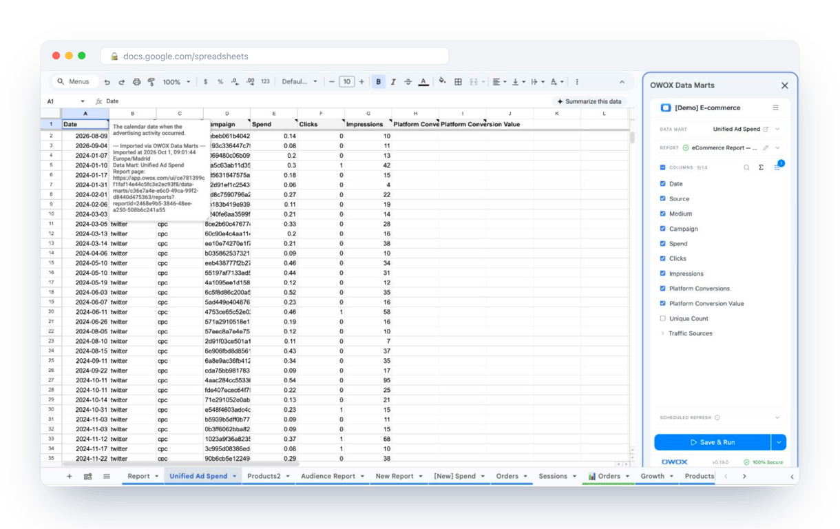
What changes for the person who maintains the sheet:
- Refresh replaces re-export. Refresh current report in the extension menu re-runs the same pull, and a scheduled refresh keeps the tab current without anyone touching it.
- The source is written on the sheet. The header cell of an imported tab carries a note with the data mart it came from, the time of the import and a link to the report.
- No SQL and no warehouse access needed. The analyst decides which data marts and columns are available. You choose from that list.
The extension does not write or change the analyst’s SQL. Everyone rounds the same refreshed numbers, and a difference between two reports is a difference in the formulas, which is easy to find. The extension comes with the OWOX Cloud plans of OWOX Data Marts; spreadsheet reporting describes both ways data reaches a sheet.
Turn your data into decisions.
Governed data marts give you the clean foundation ML needs to actually work.
- No AI hallucinations
- Analyst-governed definitions
- Every number traces to SQL
Frequently Asked Questions
Can I round negative numbers using the ROUNDUP function?
Yes, ROUNDUP rounds negative numbers away from zero, just like positive numbers. For example, =ROUNDUP(-4.5, 0) will return -5, effectively rounding the value up to the nearest integer away from zero.
What’s the difference between FLOOR and FLOOR.MATH in Google Sheets?
For positive numbers FLOOR and FLOOR.MATH return the same result: both round down to a multiple. They differ for negative numbers. FLOOR(-4.3, 1) and FLOOR.MATH(-4.3) both return -5, away from zero, but FLOOR.MATH has a third argument, mode: FLOOR.MATH(-4.3, 1, 1) returns -4, toward zero. FLOOR gets the same result with a negative factor, FLOOR(-4.3, -1).
How do I troubleshoot the #VALUE! error when using the FLOOR function in Google Sheets?
The #VALUE! error often indicates a non-numeric entry in your FLOOR formula. Check that all values and cells referenced are numbers, and remove any text or formatting that may interfere with the calculation.
How can I round numbers up to the nearest 10 in Google Sheets?
Enter =CEILING(cell, 10) to round a number up to the next multiple of 10. This is useful for standardizing figures, managing financial data, and simplifying values into rounded increments, especially when grouping data into easily readable numbers.
How do I round numbers to two decimal places in Google Sheets?
Use =ROUND(cell, 2), where "cell" is the cell reference or value you want to round. This formula ensures the value is rounded to exactly two decimal places, ideal for financial data, grades, or any other information requiring decimal precision.
What is the difference between the ROUND, FLOOR, and CEILING functions in Google Sheets?
ROUND rounds numbers to the nearest specified decimal or integer, useful for general rounding. FLOOR rounds down to the nearest multiple, ideal for budgeting or standardizing figures. CEILING rounds up to the nearest multiple, ensuring values meet or exceed set thresholds.