Dates and times in Google Sheets: how they work, with formulas
Google Sheets stores a date as a whole number and a time as a fraction of a day. This guide explains that model and shows how to combine and split date-time values, insert the current date and time, sort by date, shift time zones and measure durations.
Google Sheets stores every date as a whole number and every time as a fraction of a day. A date with a time is the two added together. Once you know that, most date and time tasks come down to simple arithmetic:
| You need | Formula |
|---|---|
| Combine a date and a time | =B3 + C3 |
| Date from a date-time | =INT(B3) |
| Time from a date-time | =MOD(B3, 1) |
| Current date and time | =NOW() |
| Add 90 minutes | =B3 + TIME(1, 30, 0) |
| Shift by a time zone offset, here 5 hours back | =B3 - 5/24 |
| Time between two date-times | =C3 - B3, formatted as a duration |
How Google Sheets stores dates and times
How Google Sheets stores dates and times
A date is a serial number: the number of days since December 30, 1899. October 1, 2024 is 45566. A time is the part of a day that has passed: 6:00 AM is 0.25, noon is 0.5, 6:00 PM is 0.75. So 12 hours are 0.5 days, and one hour is 1/24.
The format of a cell decides only how the number is shown. Change the format under Format > Number and the same value appears as a date, a time, a date-time or a plain number, while formulas keep working with the number underneath.
Arithmetic with dates
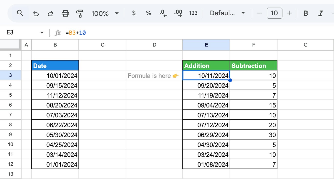
Because a day is 1, adding a number to a date moves it by that many days:
=B3+10
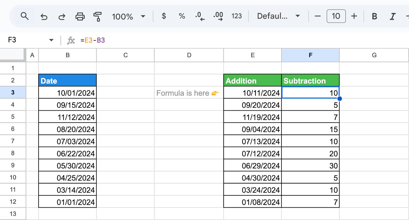
Subtracting one date from another gives the number of days between them:
=E3-B3
Arithmetic with times
To add hours and minutes, build the amount with the TIME function:
=B3+TIME(1, 30, 0)
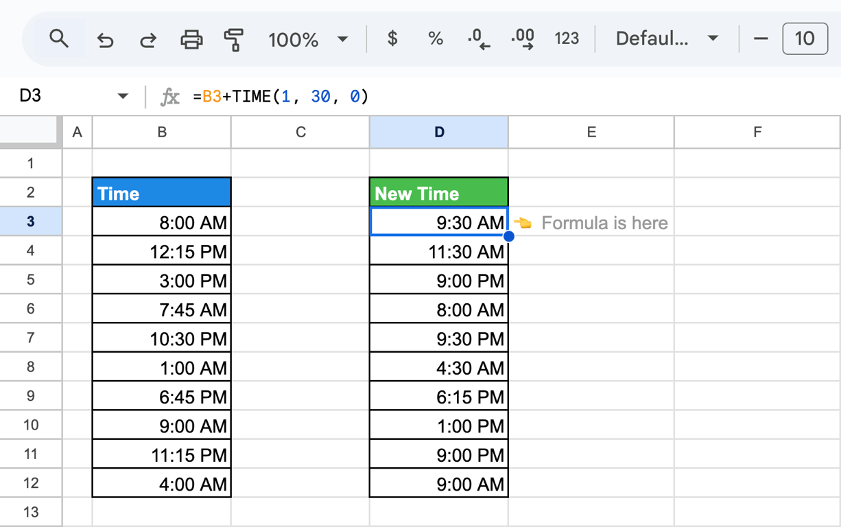
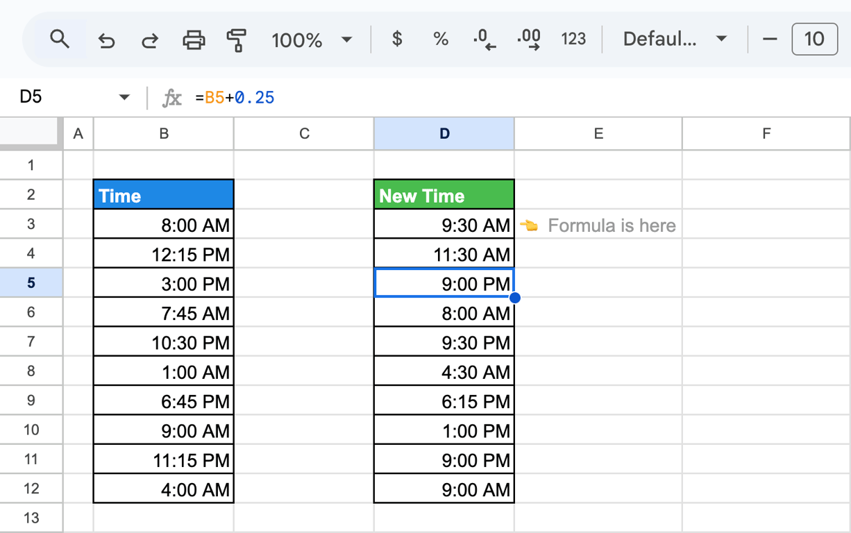
TIME(1, 30, 0) is one hour and thirty minutes, so 8:00 AM becomes 9:30 AM. The same can be written as a fraction of a day. Adding 0.25 adds six hours:
=B5+0.25
Write dates and times inside a formula
Write dates and times inside a formula
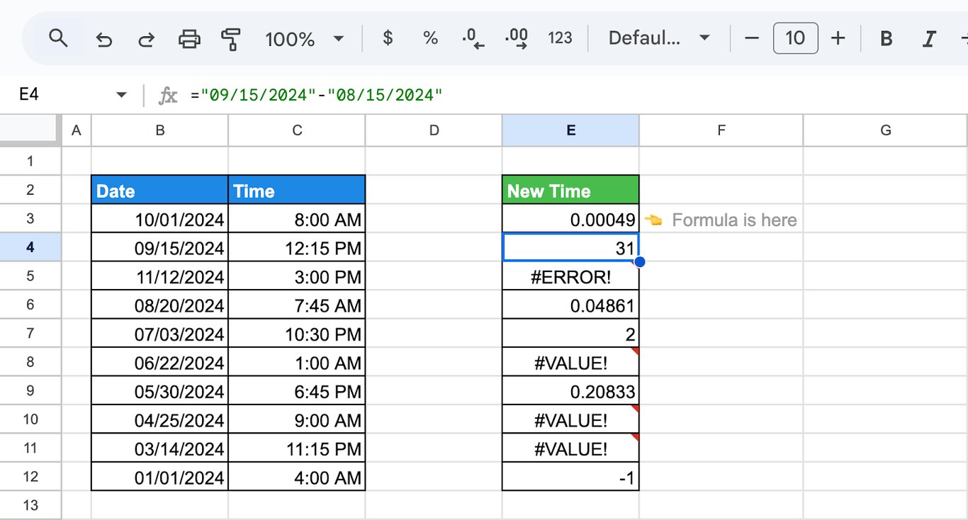
A date or a time typed straight into a formula has to be in quotes:
="09/15/2024"-"08/15/2024"
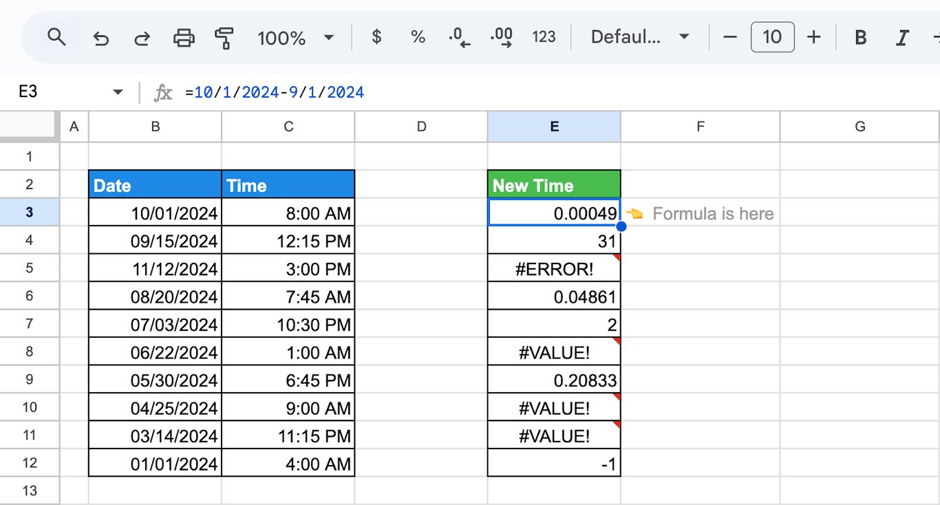
Without quotes, Sheets reads the slashes as division. =10/1/2024-9/1/2024 is calculated as 10 divided by 1 divided by 2024, minus 9 divided by 1 divided by 2024, and returns 0.00049 with no error.
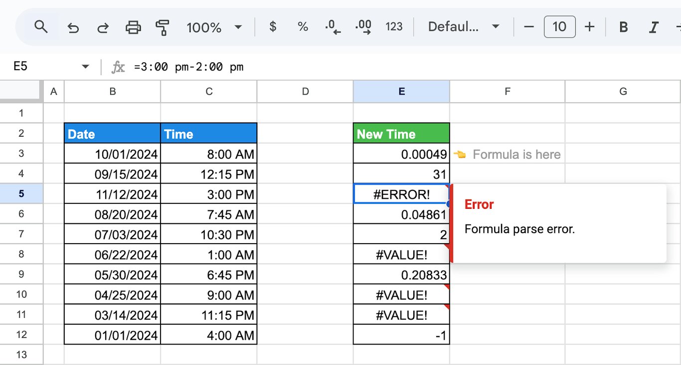
An unquoted time is not accepted at all: =3:00 pm-2:00 pm is a formula parse error.
A quoted date is read in the format of the spreadsheet locale, so “09/15/2024” works in a United States locale and fails in one that expects the day first. The DATE function has no such problem:
=DATE(2024, 7, 4)
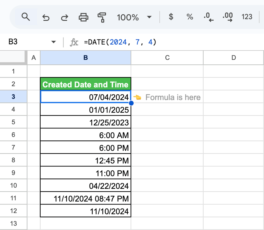
DATE(year, month, day) and TIME(hour, minute, second) return real date and time values in any locale.
OWOX Data Marts
See your first report built in real time. 15 minutes.
- Connect your data warehouse
- Pick your metrics
- Get a live Google Sheets report
In the time it takes to write a ticket. Then imagine never writing that ticket again.
Book a DemoWe'll use your actual use case
Combine a date and a time
Add them
With the date in one cell and the time in another, add the two:
=B3+C3
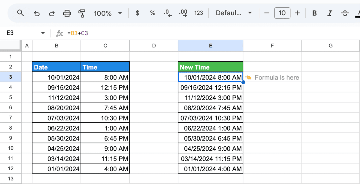
The result is a real date-time value that you can sort, compare and calculate with. If it shows only the date, apply Format > Number > Date time.
Join them as text
To get a label in a specific layout, format each part with the TEXT function and join the parts:
=CONCATENATE(TEXT(B3, "mm/dd/yyyy"), " ", TEXT(C3, "h:mm AM/PM"))
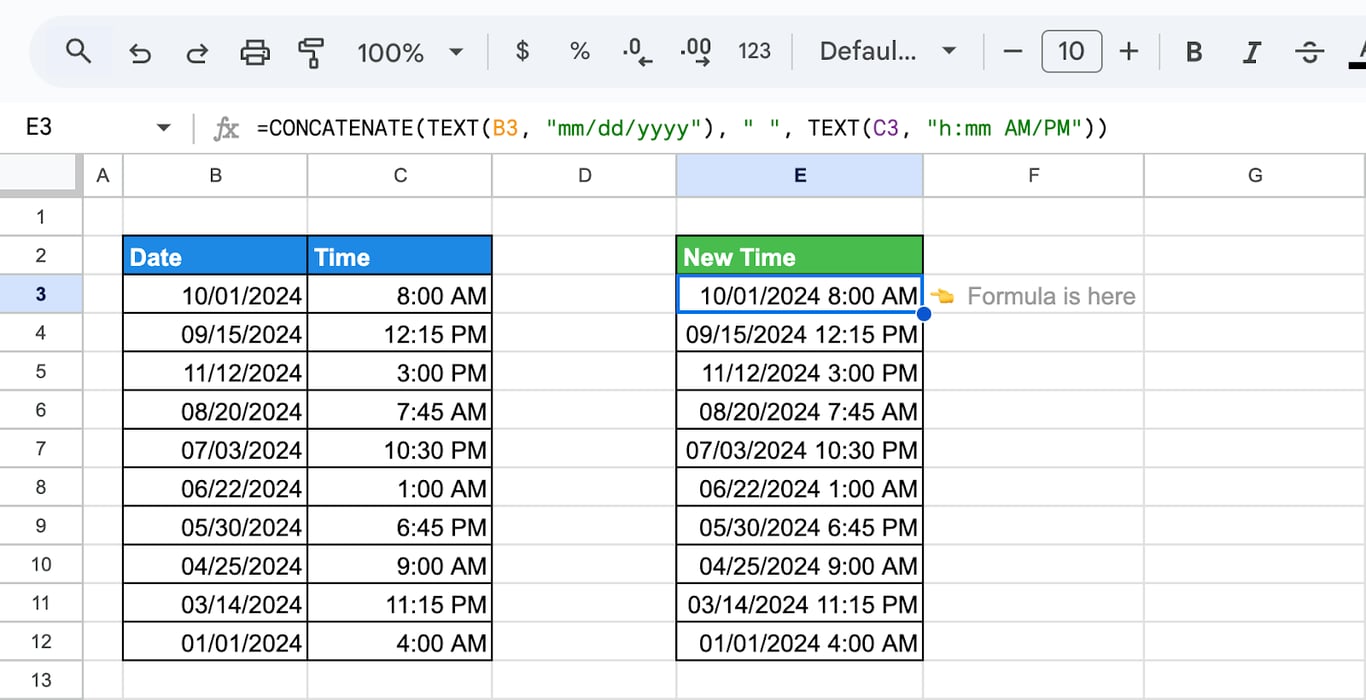
=JOIN(" ", TEXT(B3, "mm/dd/yyyy"), TEXT(C3, "h:mm AM/PM")) and =TEXT(B3, "mm/dd/yyyy") & " " & TEXT(C3, "h:mm AM/PM") return the same string. Keep in mind that the result is text: it looks like a date-time but cannot be used in date arithmetic.
Split a date-time into date and time
Split a date-time into date and time
INT for the date, the remainder for the time
The date is the whole part of the number, and INT returns it:
=INT(B3)
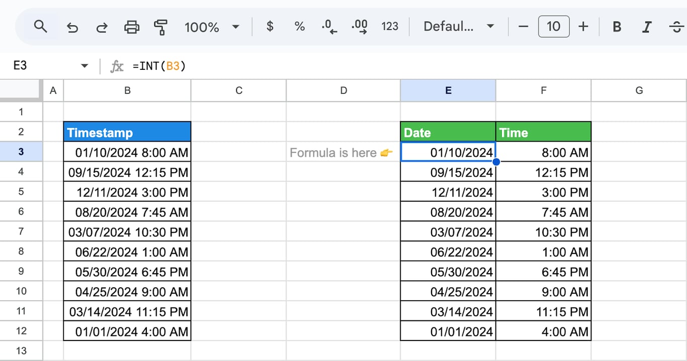
The time is what is left: =B3-E3, or in one step with MOD, which returns the fractional part:
=MOD(B3, 1)
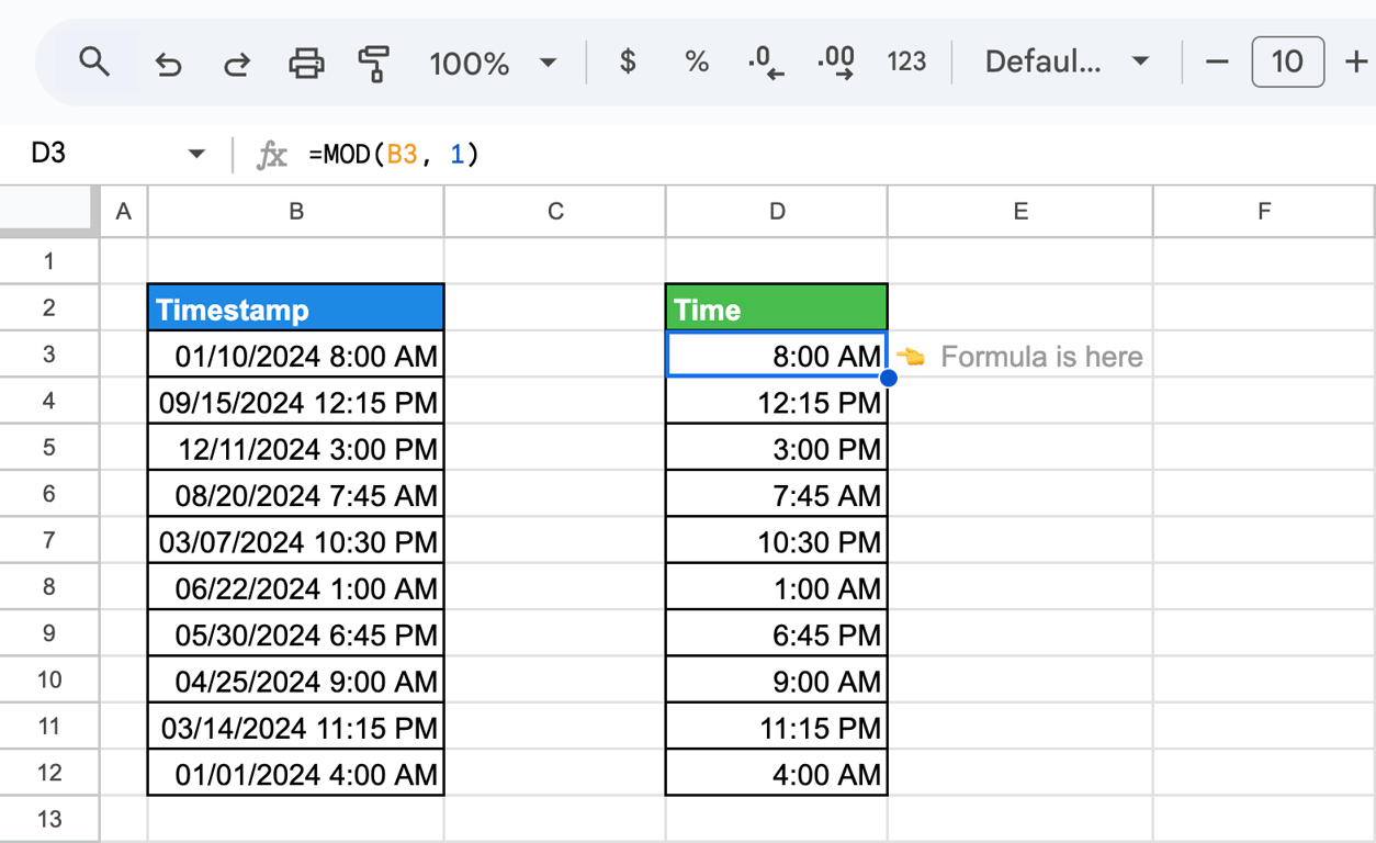
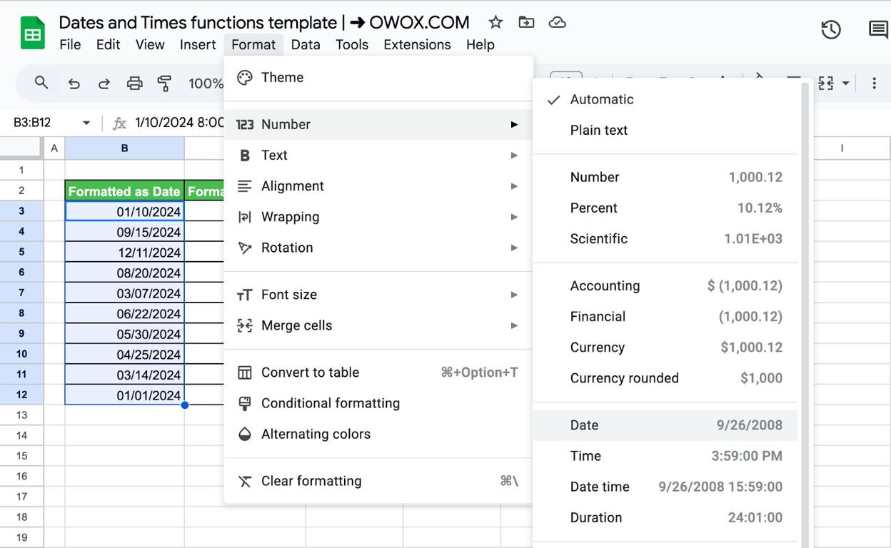
Both results are numbers. Format the date column as Date and the time column as Time under Format > Number.
TEXT for formatted text
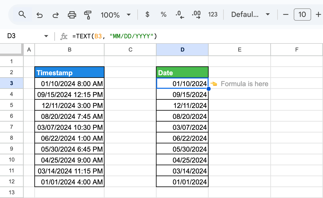
TEXT returns the part you ask for as text, in the layout you specify:
=TEXT(B3, "MM/DD/YYYY")
=TEXT(B3, "h:mm AM/PM")
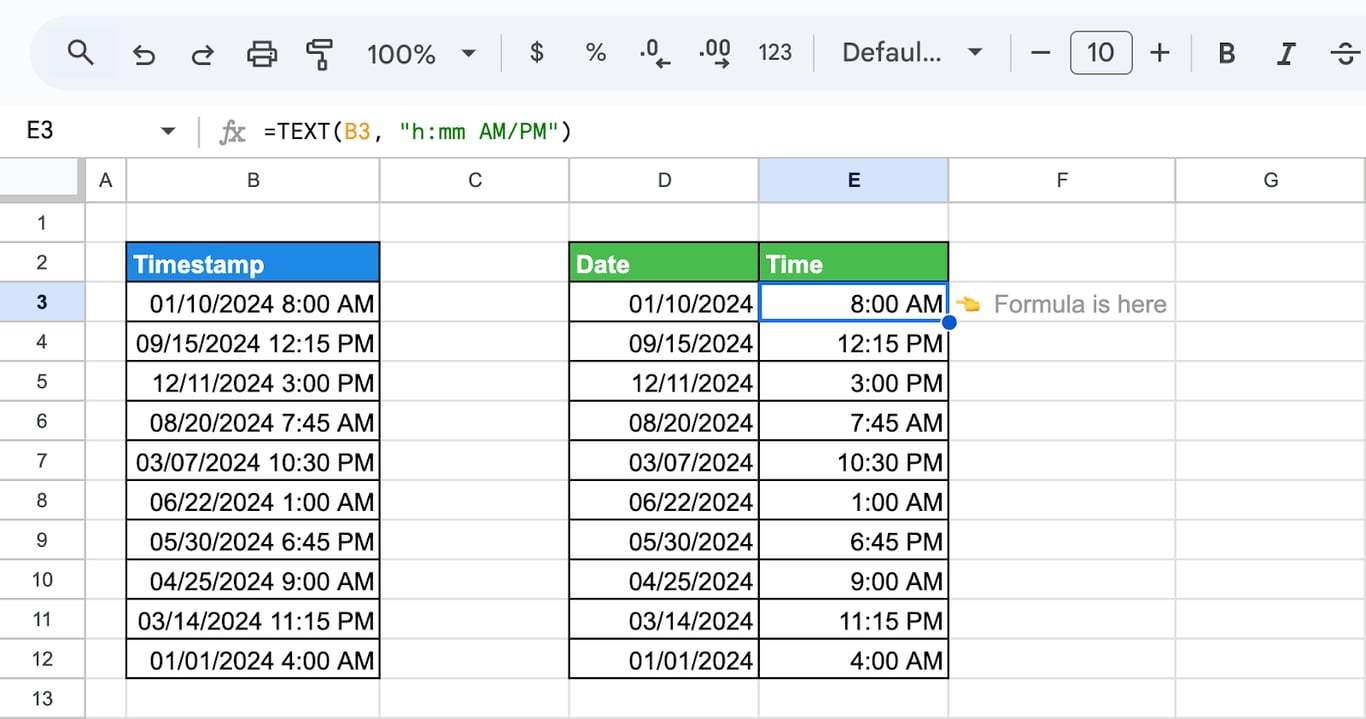
Use this for labels and exports. For further calculations, INT and MOD are the better choice, because their results stay numbers.
SPLIT for a quick separation
The SPLIT function cuts the displayed value at each space:
=SPLIT(B3, " ")
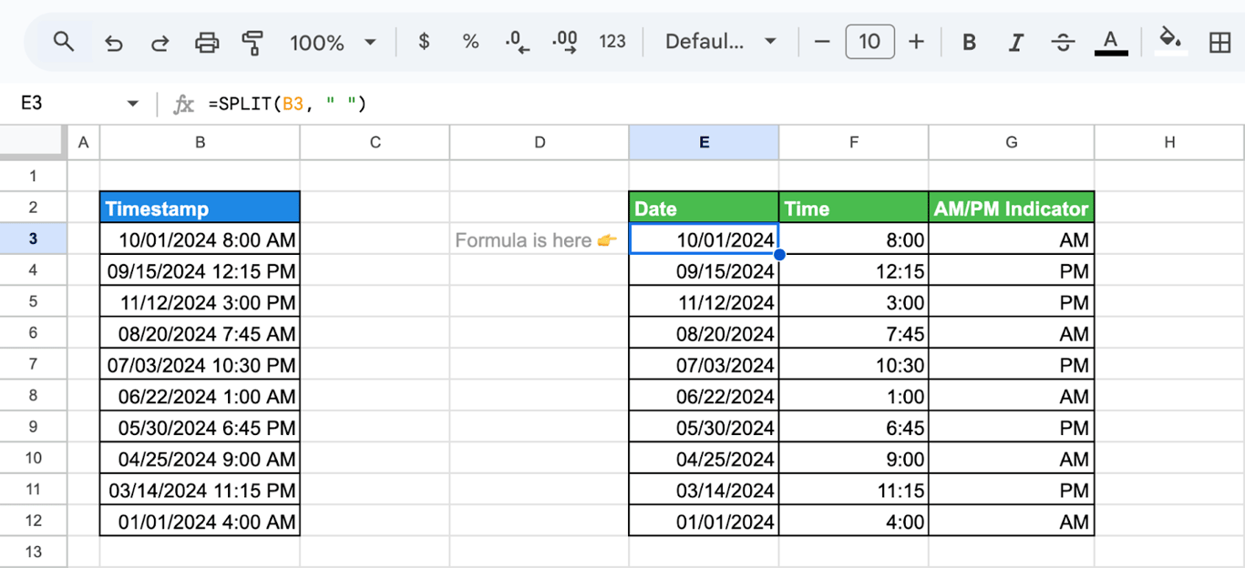
A timestamp shown as 10/01/2024 8:00 AM has two spaces, so the result has three columns: the date, the time and the AM/PM marker.
DATEVALUE and TIMEVALUE
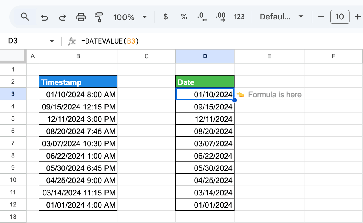
=DATEVALUE(B3)
=TIMEVALUE(B3)
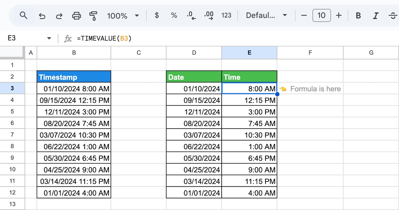
The two functions return the date and the time of a timestamp. Their main use is for dates and times that are stored as text: they convert the text into real values.
Insert the current date and time
Insert the current date and time
TODAY and NOW
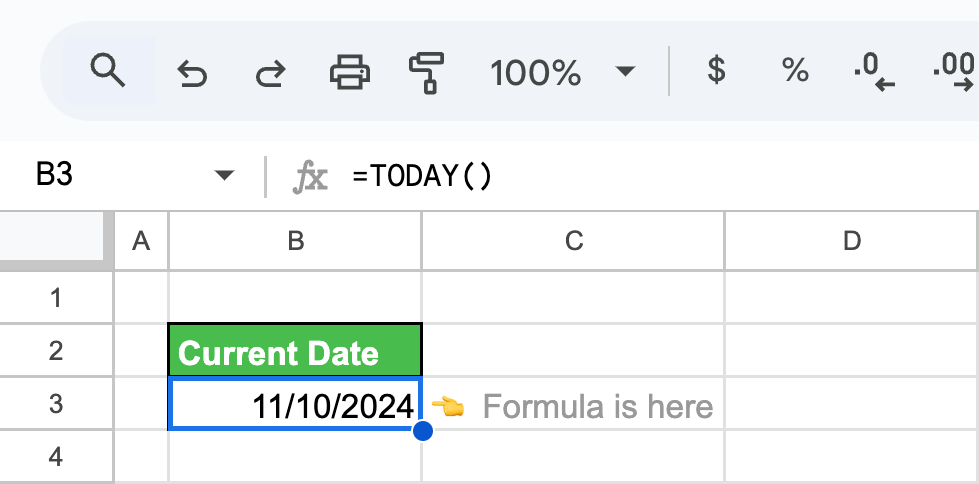
=TODAY()
=NOW()
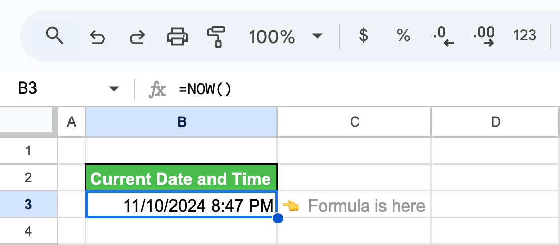
TODAY returns the current date, NOW the current date and time. Neither takes an argument, and both are recalculated when the sheet changes, so they are not suitable for recording when something happened. More in the guide to NOW and TODAY.
For the current time without the date, subtract the date part:
=NOW() - TRUNC(NOW())
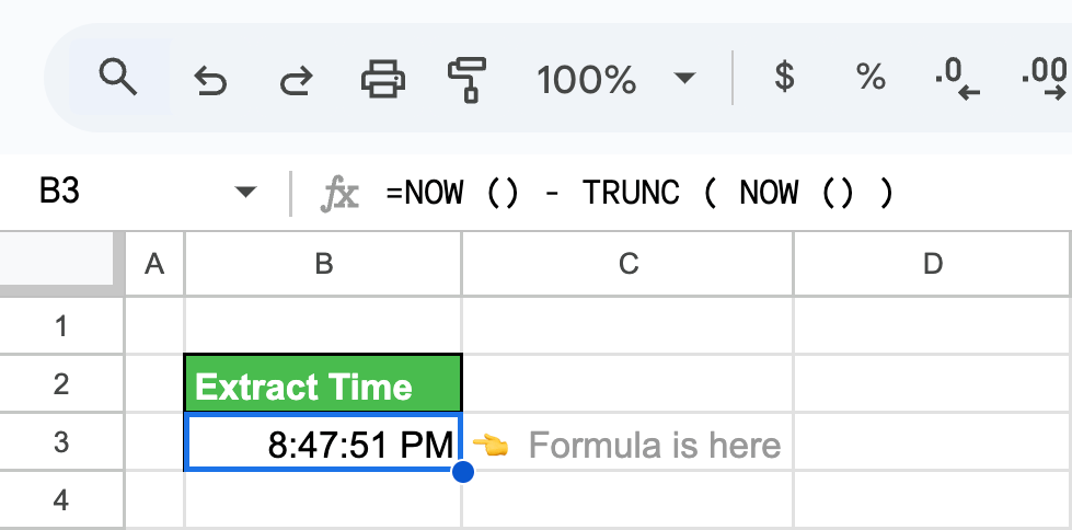
=MOD(NOW(), 1) returns the same value.
Keyboard shortcuts for a fixed date and time
A shortcut types the current value into the cell as a constant that never changes:
- Ctrl + ; (Cmd + ; on a Mac): the current date.
- Ctrl + Shift + ; (Cmd + Shift + ;): the current time.
- Ctrl + Alt + Shift + ; (Cmd + Option + Shift + ;): the current date and time.
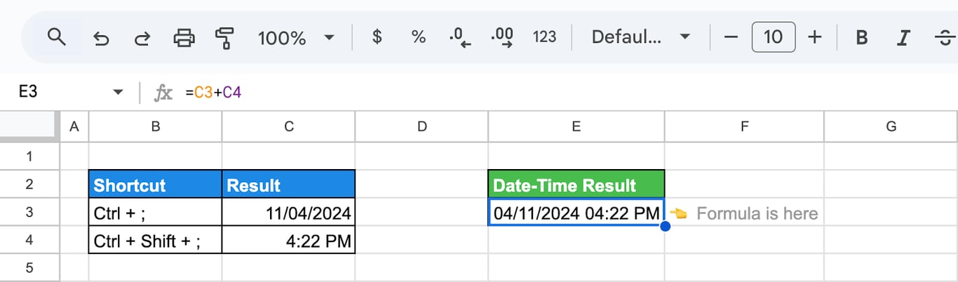
Adding the two cells, =C3+C4, gives one fixed date-time value.
A timestamp when a cell is edited
To record automatically when a row was last changed, Google Sheets needs a short script. Open Extensions > Apps Script, replace the content of the editor with the code below and save the project:
function onEdit(e) {
  if (!e) return; // Exit the function if e is undefined
  var sheet = e.source.getActiveSheet();
  var editedCell = e.range;
  var timestampColumn = 3; // Column C for the timestamp
  var targetColumn = 2; // Column B for target updates

  if (editedCell.getColumn() == targetColumn) {
    var timestampCell = editedCell.offset(0, timestampColumn - targetColumn);
    timestampCell.setValue(new Date());
  }
}- onEdit: Google Sheets runs a function with this name every time a cell is edited by hand.
- targetColumn: the column to watch, here column B.
- timestampColumn: the column that receives the timestamp, here column C.
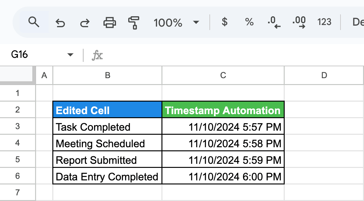
From then on, every edit in column B writes the current date and time into column C of the same row. The script applies to every tab of the file; the value it writes is fixed and does not change later.
Sort data by date
With a filter
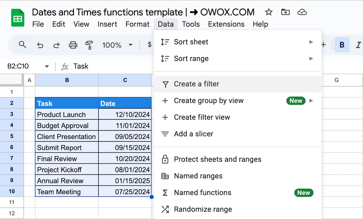
- Select the range, including the header row.
- Choose Data > Create a filter.
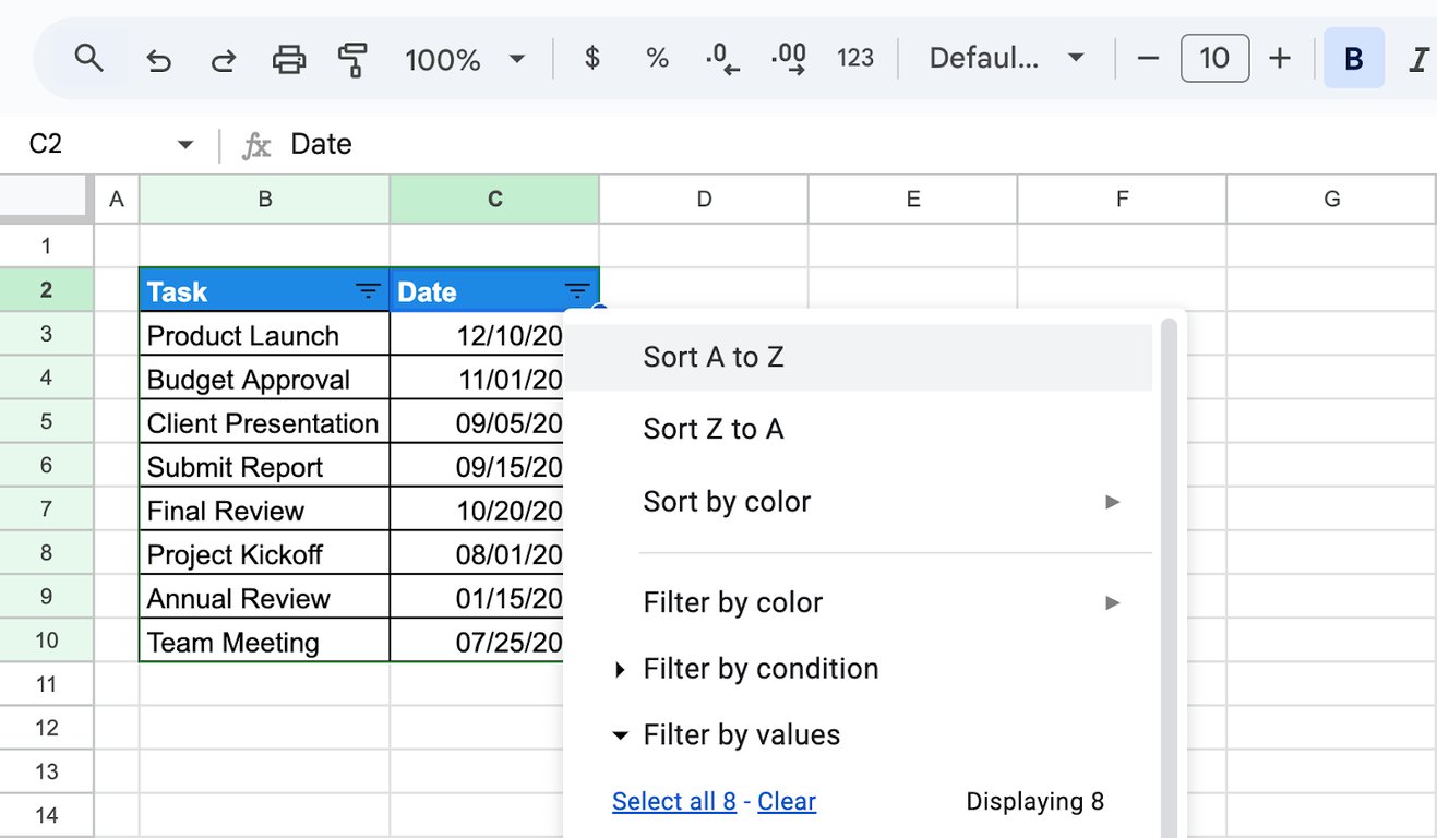
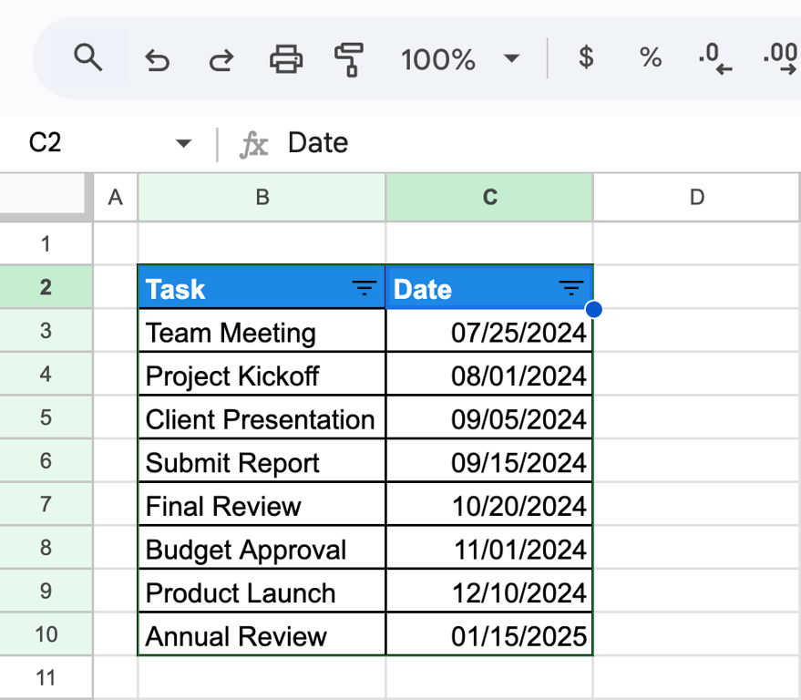
- Click the filter icon in the header of the date column and choose Sort A to Z for oldest first or Sort Z to A for newest first.
With the SORT function
The SORT function returns a sorted copy and leaves the original range as it is:
=SORT(B3:C10, 2, TRUE)
- B3:C10: the range with tasks and dates.
- 2: sort by the second column of the range, the dates.
- TRUE: ascending order, oldest first. FALSE reverses it.
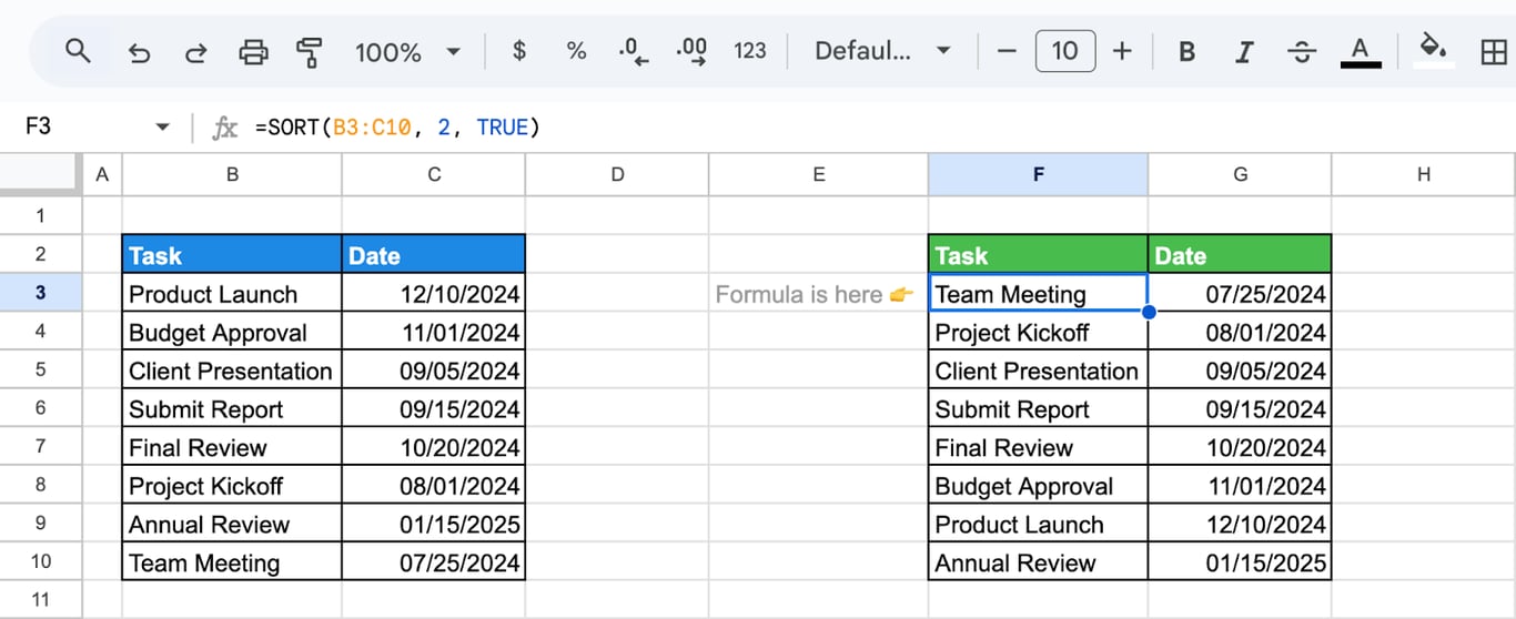
The copy updates by itself when the source data changes.
With sort range
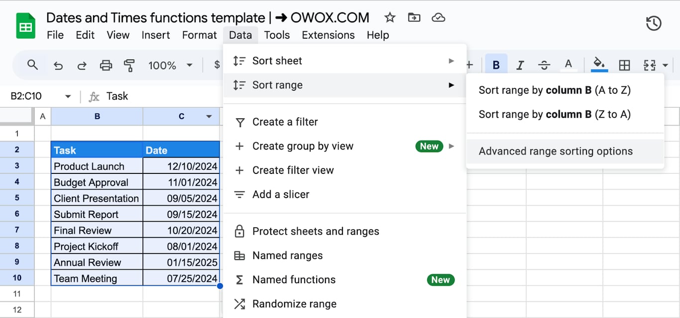
- Select the rows to sort, here B3:C10.
- Choose Data > Sort range > Advanced range sorting options.
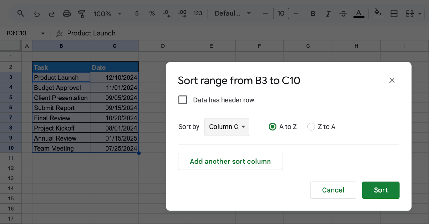
- Pick the date column under Sort by, choose A to Z or Z to A and click Sort. If the selection includes the header, tick Data has header row.
The whole sheet
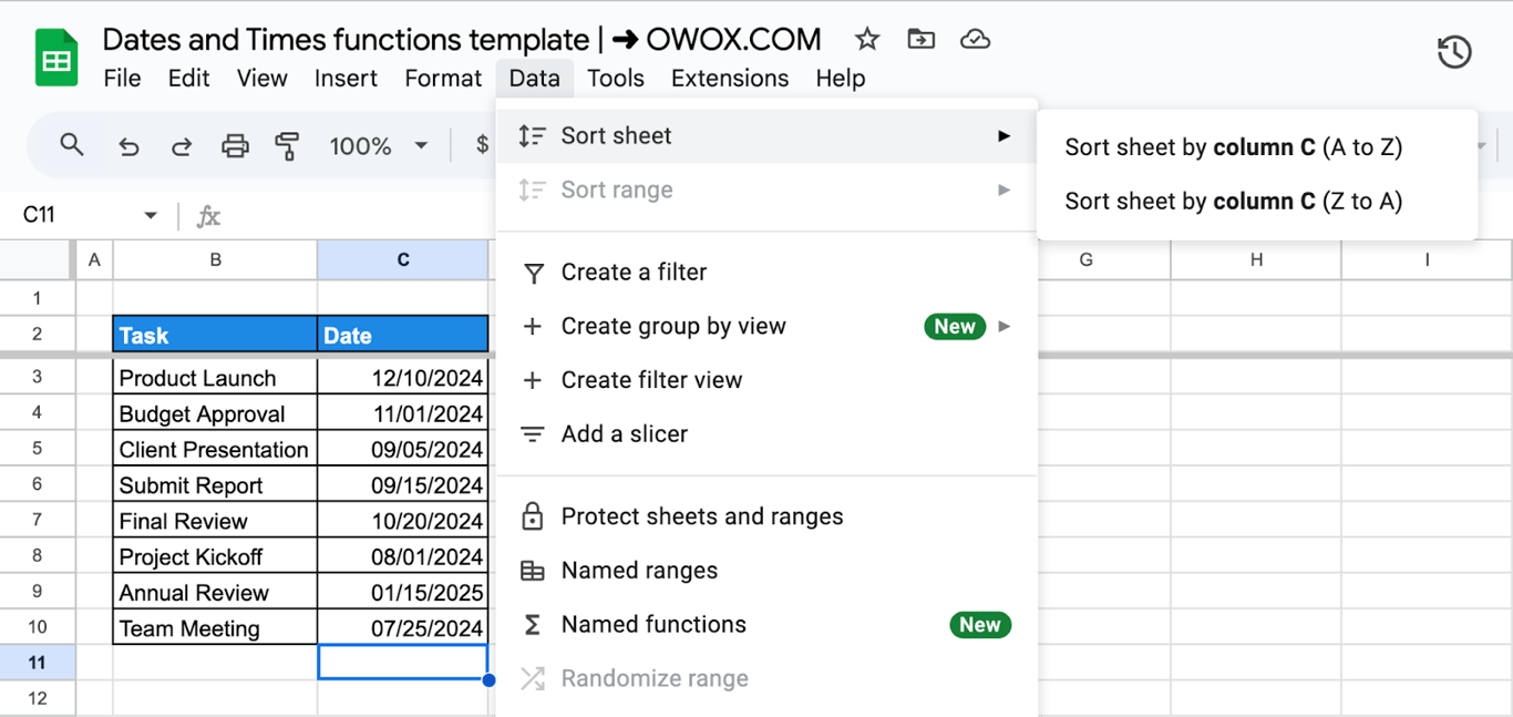
To sort every row of the tab by the date column, freeze the header row first (View > Freeze > 1 row), click any cell in the date column and choose Data > Sort sheet > Sort sheet by column (A to Z).
When the dates sort in the wrong order
⚠️ Error: Some dates end up in the wrong place, usually together at the top or the bottom.
✅ Solution: Those dates are stored as text. A text date is left-aligned by default and does not change when you apply another date format. Convert it with =DATEVALUE(B3) or retype it, then sort again. Changing the cell format alone does not turn text into a date.
Convert between time zones
Sheets has no time zone function. A conversion is a shift by the number of hours between the two zones, and one hour is 1/24 of a day.
Subtract or add the offset
To convert a UTC timestamp to a zone that is five hours behind:
=TEXT(B3 - 5/24, "yyyy-mm-dd hh:mm AM/PM")
- B3 - 5/24: the timestamp minus five hours.
- TEXT(…, “yyyy-mm-dd hh:mm AM/PM”): shows the result in a fixed layout, as text.
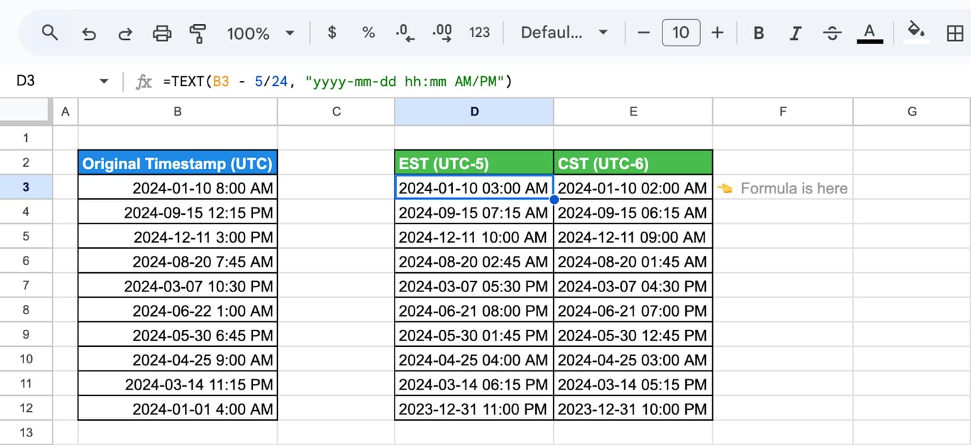
For a zone ahead of UTC, add instead: =B3 + 3/24. Leave TEXT out when you need a value you can keep calculating with.
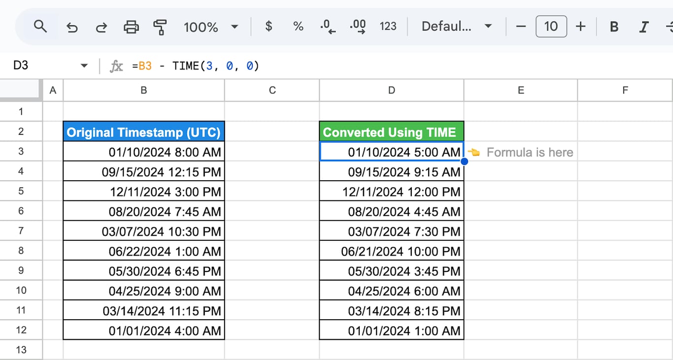
The same shift can be written with TIME:
=B3 - TIME(3, 0, 0)
Or with CONVERT, which turns hours into days:
=B3 + CONVERT(-3, "hr", "day")
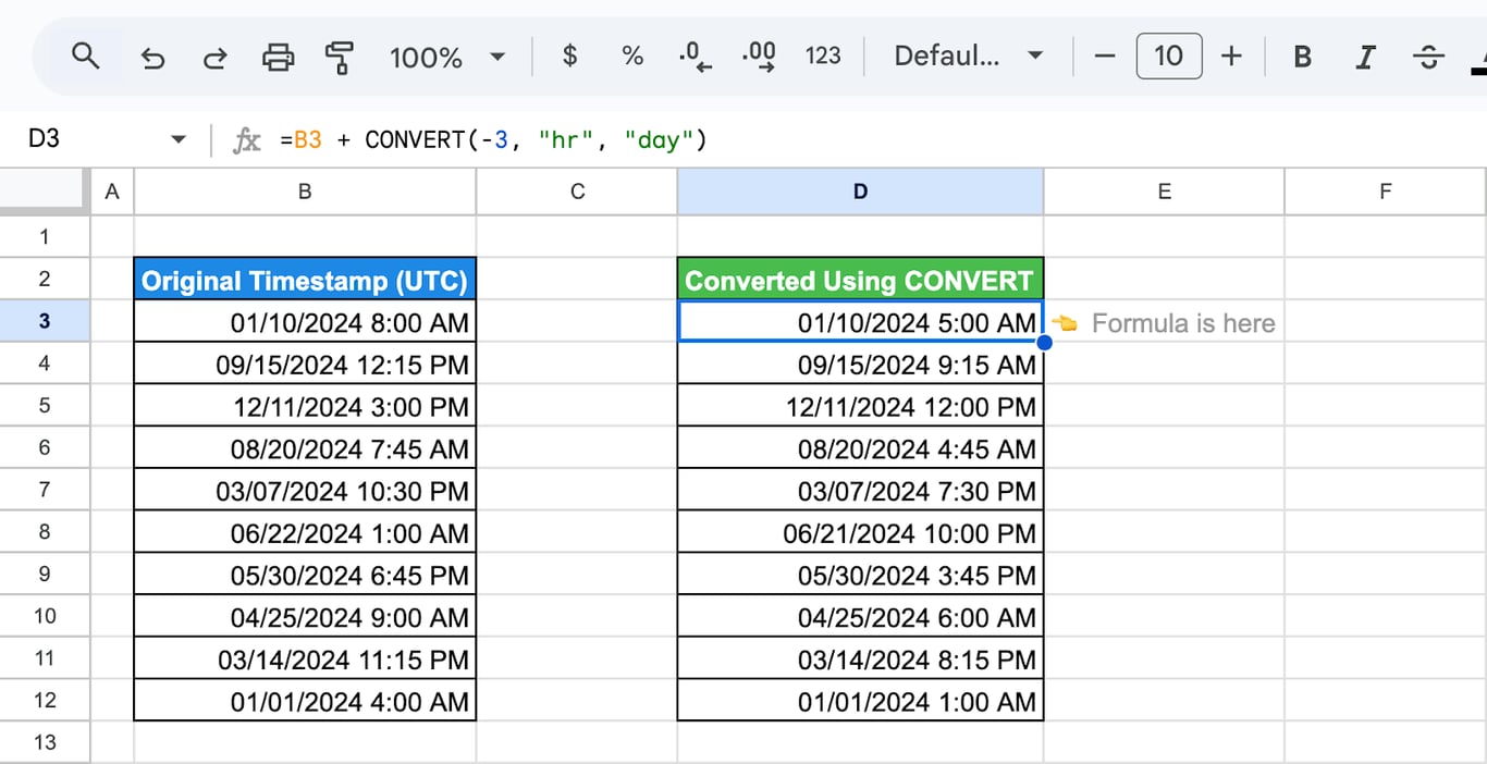
All three handle the change of date correctly: 1:00 AM minus three hours becomes 10:00 PM of the previous day.
A fixed offset ignores daylight saving time. New York is five hours behind UTC in winter and four in summer, so a formula with a constant offset is right only for part of the year.
A different zone in each row
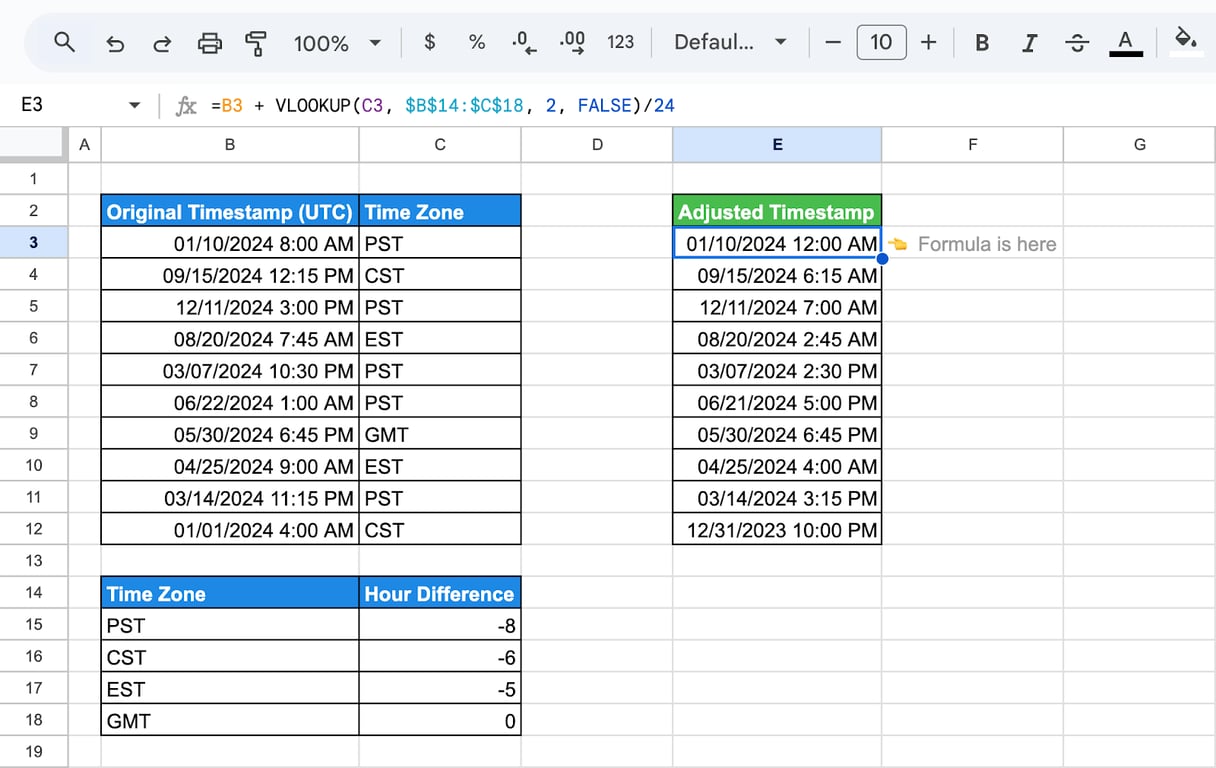
With the zone of each row in a column, keep the offsets in a small table and look them up with VLOOKUP:
=B3 + VLOOKUP(C3, $B$14:$C$18, 2, FALSE)/24
- B3: the UTC timestamp.
- VLOOKUP(C3, $B$14:$C$18, 2, FALSE): the offset in hours for the zone named in C3.
- /24: turns the hours into a fraction of a day.
Measure the time between two date-times
Measure the time between two date-times
Subtract the start from the end:
=C3-B3
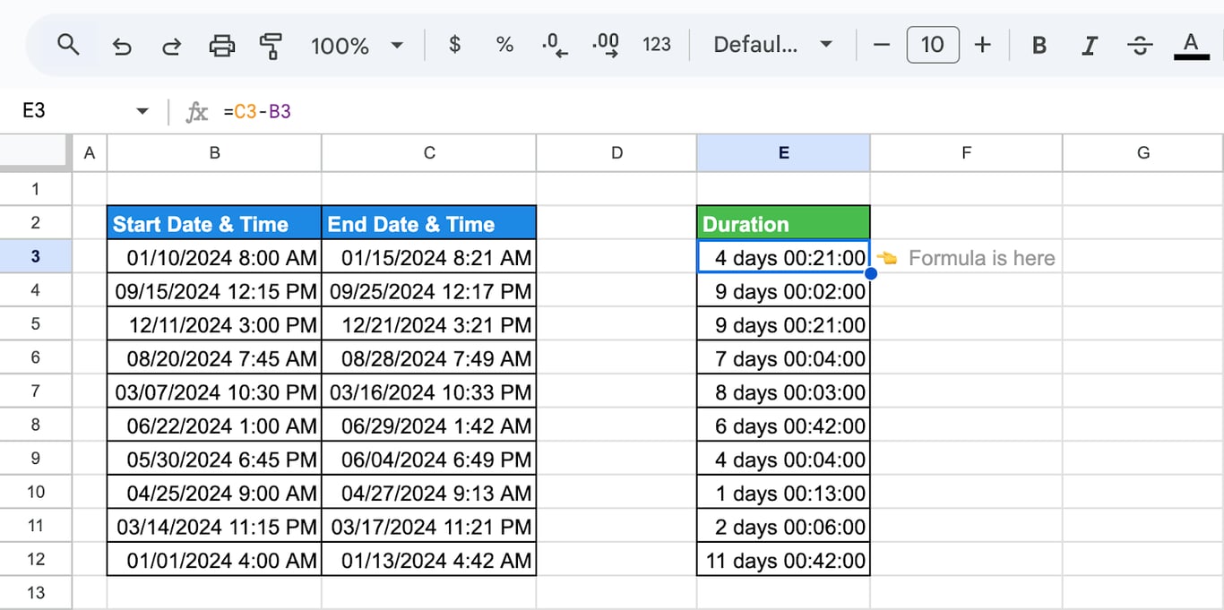
The result is a number of days with a fraction. Format it with Format > Number > Duration to see elapsed hours, minutes and seconds, or multiply it: =(C3-B3)*24 gives the difference in hours as a plain number.
When the two timestamps were recorded in different time zones, bring one of them to the zone of the other first, then subtract:
=D3-B3
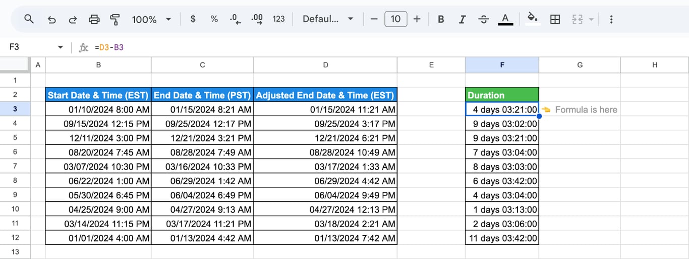
Here column D holds the end time shifted to the time zone of the start time.
Related Google Sheets functions
Related Google Sheets functions
Functions that are often used with dates and times, each with its own guide:
- DATE functions: DATE, EDATE, DATEVALUE and DATEDIF for building and comparing dates.
- TIME functions: TIME, HOUR, MINUTE and SECOND, and time arithmetic.
- NOW and TODAY: The current date and time.
- WEEKDAY/WEEKNUM: Returns the day of the week or the week number of the year for a date, useful for weekly reporting.
- MONTH/EOMONTH: Extracts the month from a date or returns the last day of a month, handy for monthly reports.
- WORKDAY and NETWORKDAYS: Working days between dates.
- TEXT: Converts numbers and dates into text in the format you specify.
- QUERY date filtering: Filters rows by a date or a date range inside a QUERY formula.
Clean dates start before the sheet
Clean dates start before the sheet
Most date problems in a spreadsheet are not formula problems. They come with the data: one export writes 10/01/2024, another 2024-10-01 as text, a third one is in UTC while the rest is in local time. Every fix in this guide, from DATEVALUE to time zone offsets, repairs something that was already inconsistent when it was pasted in.
The OWOX Data Marts extension for Google Sheets covers that half. A data analyst publishes a data mart (a table or an SQL query in your data warehouse) and makes it available for reports. In Sheets you open the extension, pick the data mart, tick the columns you want and run it. The rows land in a tab, ready for your formulas.
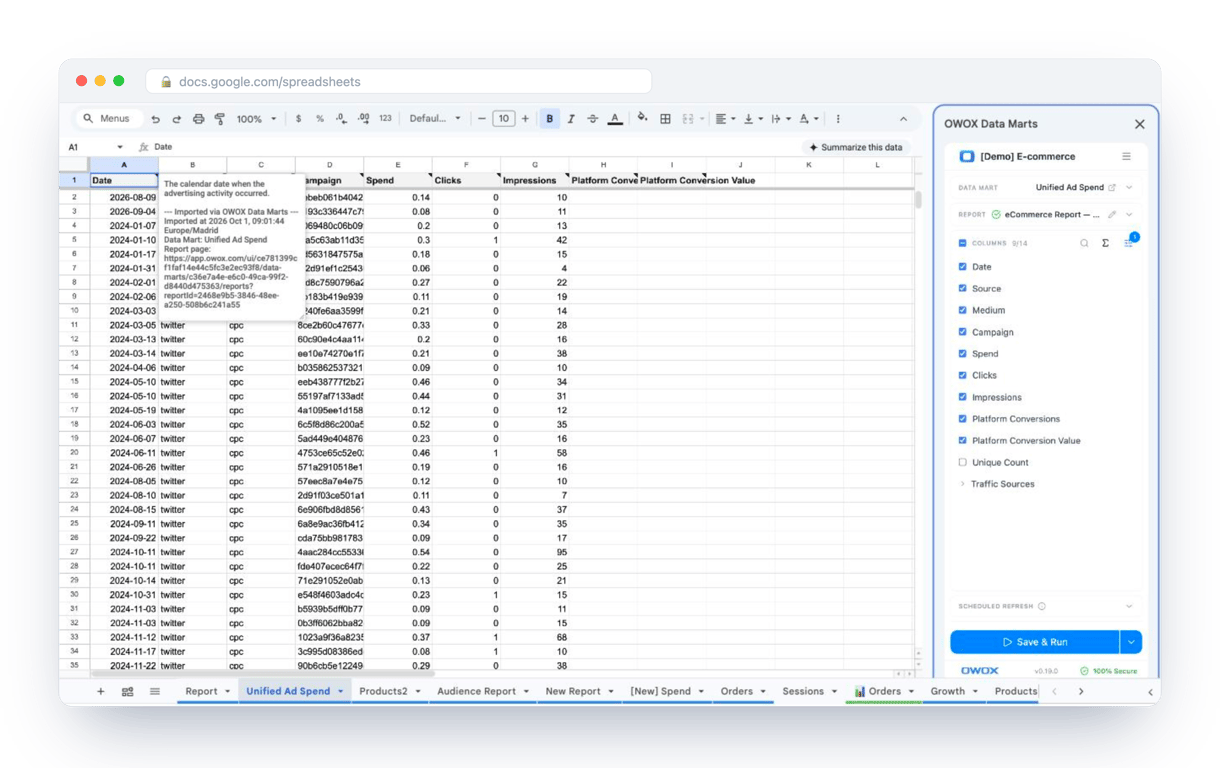
What changes for the person who maintains the sheet:
- Refresh replaces re-export. Refresh current report in the extension menu re-runs the same pull, and a scheduled refresh keeps the tab current without anyone touching it.
- The source is written on the sheet. The header cell of an imported tab carries a note with the data mart it came from, the time of the import and a link to the report.
- No SQL and no warehouse access needed. The analyst decides which data marts and columns are available. You choose from that list.
The extension does not write or change the analyst’s SQL. Formats and time zones are settled there once, and the sheet receives the same columns in the same form on every refresh. The extension comes with the OWOX Cloud plans of OWOX Data Marts; spreadsheet reporting describes both ways data reaches a sheet.
Turn your data into decisions.
Governed data marts give you the clean foundation ML needs to actually work.
- No AI hallucinations
- Analyst-governed definitions
- Every number traces to SQL
Frequently Asked Questions
Can I automate the insertion of a timestamp when editing a cell in Google Sheets?
Yes, you can automate the insertion of a timestamp when editing a cell in Google Sheets by using Google Apps Script. Create a script that triggers on edit, capturing the current date and time, and inserting it into a specified cell or column whenever a change occurs.
What’s the easiest way to split date and time into separate columns?
Use =INT(A1) for the date and =MOD(A1, 1) for the time, where A1 holds the date-time value, then format the first result as Date and the second as Time. Both results stay real values that you can sort and calculate with. For text output, use =TEXT(A1, "mm/dd/yyyy") and =TEXT(A1, "h:mm AM/PM").
How can I sort data by date in Google Sheets?
To sort data by date in Google Sheets, select the range of cells containing your data. Then, click on "Data" in the menu and choose "Sort range". Select the column with the dates and specify whether to sort in ascending or descending order, then click "Sort".
How do I convert a timestamp to a different time zone in Google Sheets?
To convert a timestamp to a different time zone in Google Sheets, use the formula =A1 + (TIMEZONE_OFFSET/24), where A1 contains the original timestamp and TIMEZONE_OFFSET is the difference in hours between the original and target time zones. Format the result as a date-time for clarity.
How do I automatically insert the current date or time in Google Sheets?
To automatically insert the current date in Google Sheets, use the formula =TODAY(). For the current time, use =NOW(). These functions update automatically with changes to the spreadsheet, providing the most current date and time without manual input.
How can I combine date and time in Google Sheets?
To combine date and time in Google Sheets, utilize the formula =A1 + B1, where A1 represents the cell containing the date and B1 contains the time. Ensure the resulting cell is formatted as a date-time format by navigating to Format > Number > Date time for proper display.