HLOOKUP in Google Sheets: syntax, examples and errors
HLOOKUP searches for a key in the first row of a range and returns the value from another row of the same column. This guide covers the syntax, exact and approximate match, finding the row with MATCH, two-way lookups, the XLOOKUP and INDEX with MATCH alternatives, and what each HLOOKUP error means.
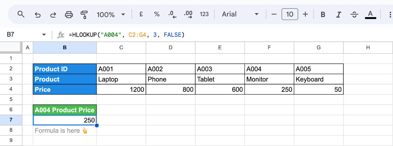
HLOOKUP searches for a value in the first row of a range and returns the value from another row of the same column:
=HLOOKUP("A004", C2:G4, 3, FALSE)
The formula finds “A004” in the first row of C2:G4 and returns what is in the third row of that column. It is VLOOKUP turned on its side: use it when the keys run across the top of the table and the attributes run down.
HLOOKUP syntax
=HLOOKUP(search_key, range, index, [is_sorted])
- search_key: the value to look for.
- range: the table. The key is searched in its first row.
- index: the number of the row to return, counted from the top of the range. 1 is the first row itself.
- is_sorted: FALSE for an exact match. TRUE, the default, assumes the first row is sorted in ascending order and returns the nearest match that is not greater than the key.
Set the last argument to FALSE unless you need the approximate match. Left out, it is TRUE, and on an unsorted row that returns wrong values or #N/A.
| HLOOKUP | VLOOKUP | |
|---|---|---|
| Searches in | The first row of the range | The first column of the range |
| Returns from | A row, by number | A column, by number |
| Fits tables where | Each record is a column | Each record is a row |
Most data is stored with one record per row, which is why VLOOKUP is far more common. HLOOKUP is for the tables that are laid out the other way: months across the top, plans or products as columns.
Examples
Return another row
=HLOOKUP("A003", C2:G4, 3, FALSE)
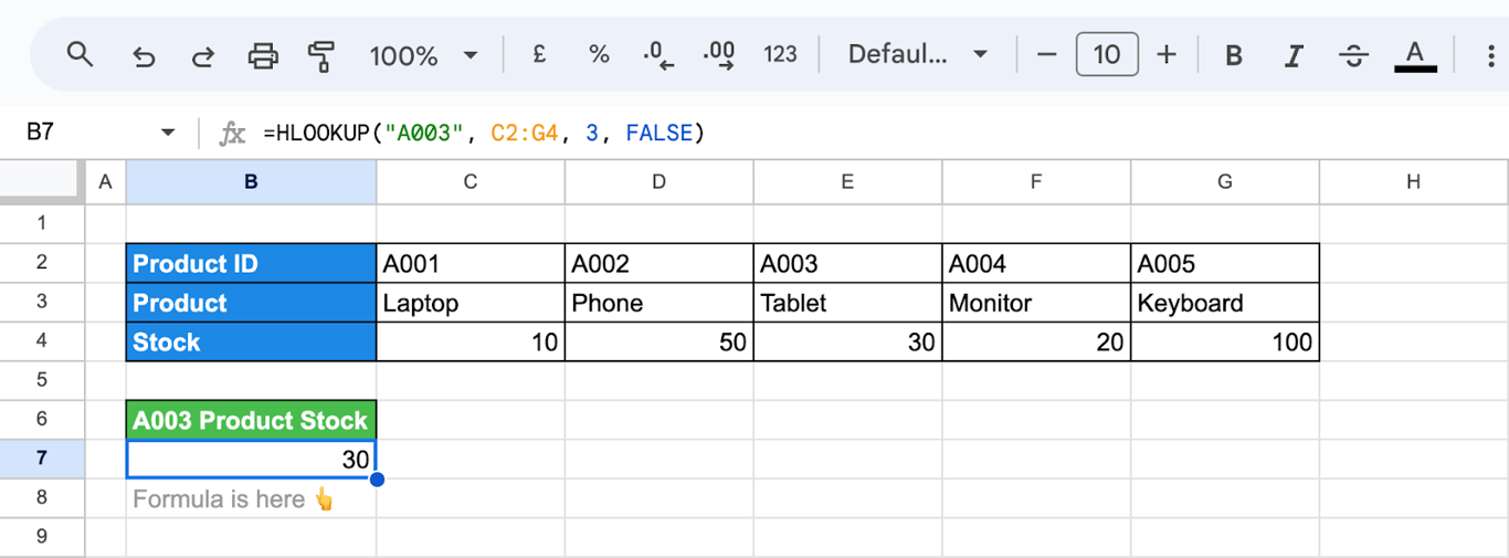
The index 3 points to the third row of the range, the stock. Change it to 2 for the product name.
The key occurs twice
=HLOOKUP("A003", C2:G4, 2, FALSE)
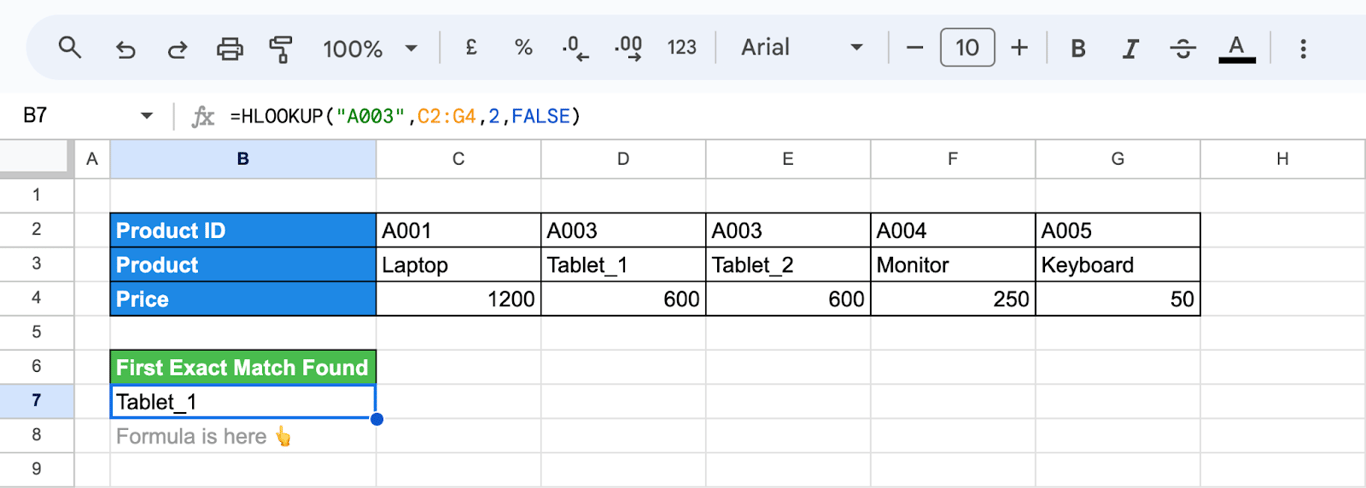
HLOOKUP returns the first match from the left and ignores the rest, without a warning. If keys can repeat, check them with COUNTIF before trusting the lookup.
Approximate match
With TRUE as the last argument, HLOOKUP looks for the largest value in the first row that is less than or equal to the key. That works only when the row is sorted in ascending order.
=HLOOKUP(300, C3:G4, 2, TRUE)
On a row sorted from high to low, the formula returns #N/A:
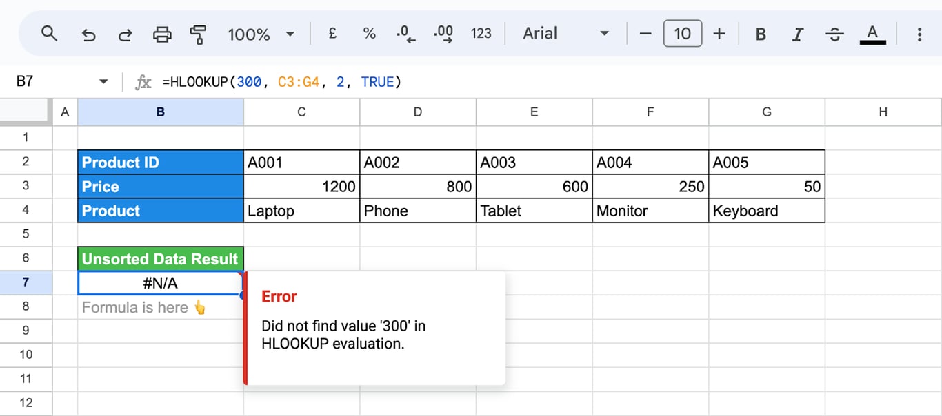
With the same prices in ascending order, it returns the product at 250, the highest price that does not exceed 300:
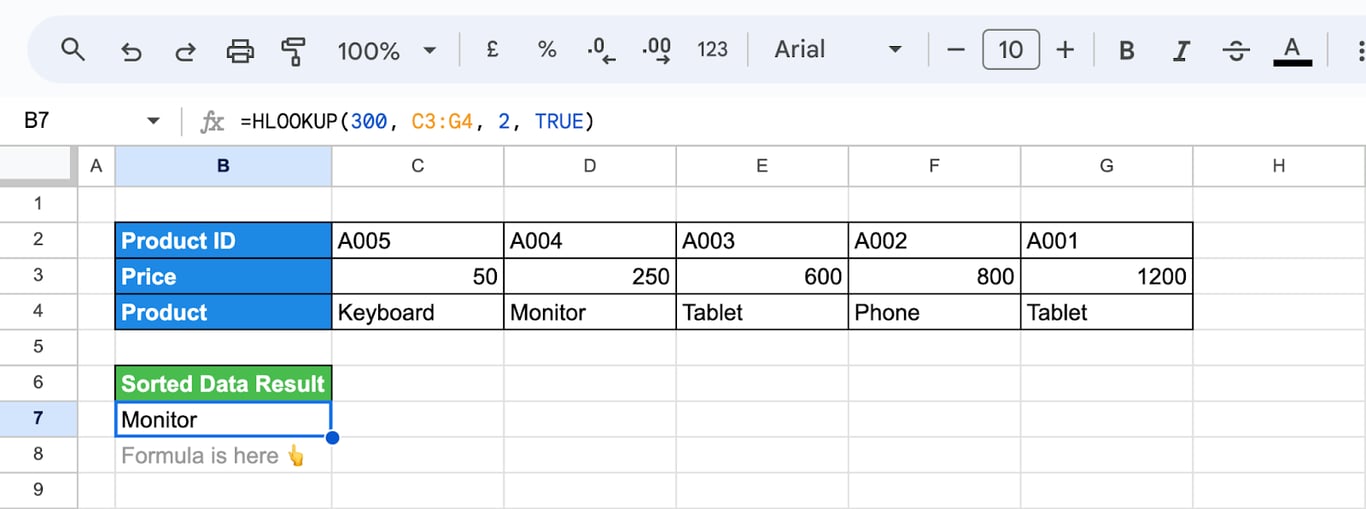
The approximate match is the tool for brackets: discount tiers, tax bands, grade boundaries written across a row.
Wildcards
With an exact match, the key can contain an asterisk for any text and a question mark for one character: =HLOOKUP("A00*", C2:G4, 2, FALSE) returns the value under the first ID that starts with “A00”. Text matching is not case-sensitive.
OWOX Data Marts
See your first report built in real time. 15 minutes.
- Connect your data warehouse
- Pick your metrics
- Get a live Google Sheets report
In the time it takes to write a ticket. Then imagine never writing that ticket again.
Book a DemoWe'll use your actual use case
Find the row with MATCH
A row number typed into the formula breaks when a row is inserted above it. MATCH finds the number by the row label:
=HLOOKUP("A003", C2:G5, MATCH("Stock", B2:B5, 0), FALSE)
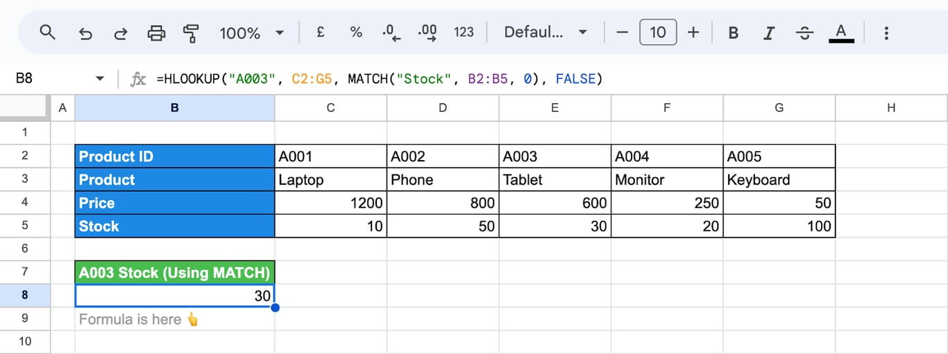
MATCH returns 4, the position of “Stock” in B2:B5, and HLOOKUP returns the fourth row of the range. Put the label in a cell and the reader can choose which attribute to see. The label range and the lookup range must start in the same row, or the numbers do not line up.
A whole column for a key
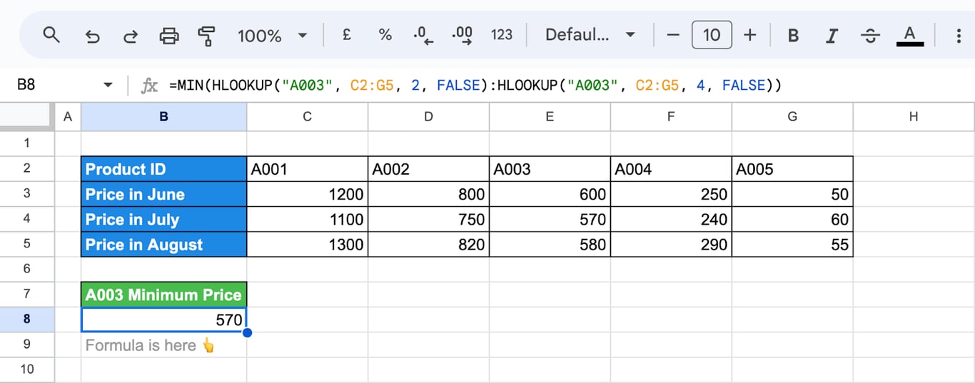
To aggregate all values of one column, such as the prices of a product over three months, pick the column with INDEX and pass it to the function:
=MIN(INDEX(C3:G5, 0, MATCH("A003", C2:G2, 0)))
The row number 0 tells INDEX to return every row of the column that MATCH found. Replace MIN with AVERAGE, MAX or SUM as needed.
The screenshot does the same with two HLOOKUP results joined by a colon into a range:
=MIN(HLOOKUP("A003", C2:G5, 2, FALSE):HLOOKUP("A003", C2:G5, 4, FALSE))
Alternatives to HLOOKUP
XLOOKUP
XLOOKUP takes the row to search and the row to return as two separate ranges, so there is no index to count and no first-row rule:
=XLOOKUP("A003", C2:G2, C4:G4)
Its fourth argument is the value to show when nothing is found: =XLOOKUP("A006", C2:G2, C4:G4, "Not found"). See XLOOKUP and VLOOKUP.
INDEX and MATCH
For a two-way lookup, by a column key and a row label at once, INDEX with two MATCH functions is the clearest form:
=INDEX(C3:G5, MATCH("Stock", B3:B5, 0), MATCH("A003", C2:G2, 0))
The first MATCH finds the row, the second the column, and INDEX returns the cell where they cross.
Handle a missing key
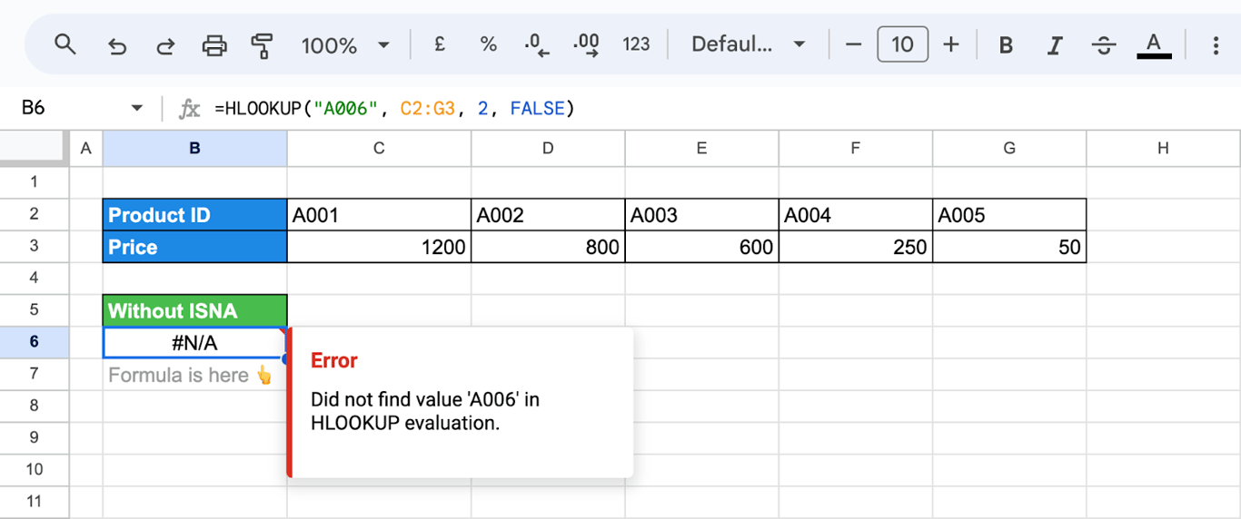
When the key is not in the first row, HLOOKUP returns #N/A:
Wrap the formula to show a text of your choice:
=IFERROR(HLOOKUP("A006", C2:G3, 2, FALSE), "Product not found")
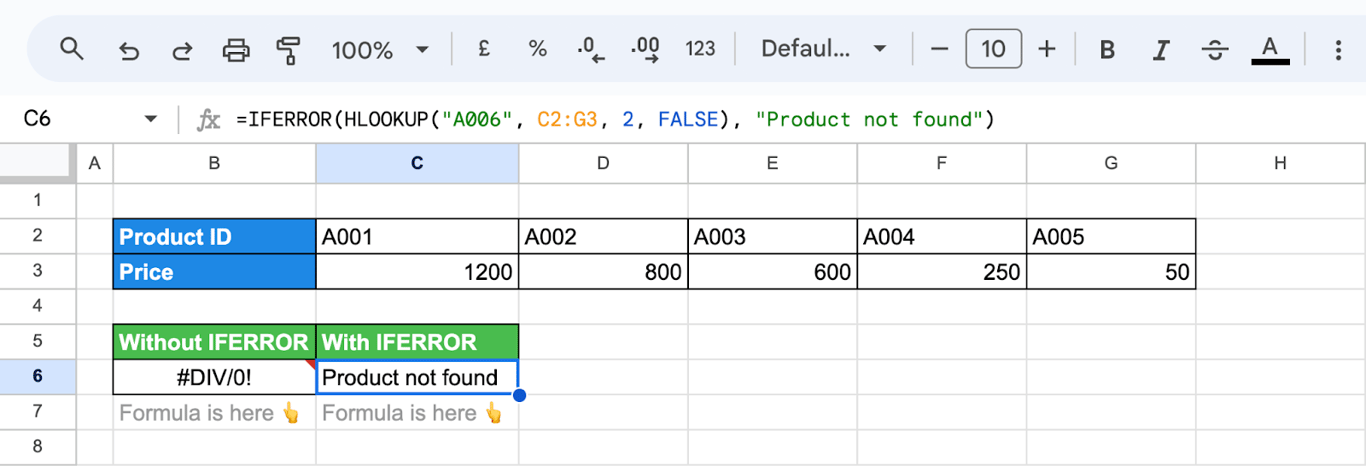
IFERROR hides every error, including a typo in the range. IFNA catches only the “not found” case and lets real mistakes show: =IFNA(HLOOKUP("A006", C2:G3, 2, FALSE), "Product not found").
HLOOKUP errors
⚠️ Error: #N/A
✅ Solution: The key is not in the first row. Check for spaces around the key or the headers, and for numbers stored as text on one side: the number 2 does not match the text “2”. With an approximate match, #N/A also means the key is smaller than every value in the row, or the row is not sorted.
⚠️ Error: #REF!
✅ Solution: The index is larger than the number of rows in the range. A range of three rows has no row 4.
⚠️ Error: #VALUE!
✅ Solution: The index is 0 or negative. Rows are counted from 1.
⚠️ Error: A wrong value, without any error.
✅ Solution: The last argument is TRUE or missing and the first row is not sorted. Add FALSE.
⚠️ Error: The formula returns values from the wrong row after the table was edited.
✅ Solution: A row was inserted and the typed index now points elsewhere. Replace the number with MATCH.
⚠️ Error: The lookup fails after the formula is copied.
✅ Solution: The range moved with the formula. Lock it with dollar signs: $C$2:$G$4.
Related guides
- VLOOKUP: The vertical lookup.
- XLOOKUP and VLOOKUP: The newer lookup function.
- LOOKUP: Approximate lookups in a row or a column.
- MATCH: The position of a value in a range.
- VLOOKUP with multiple criteria: Lookups by two or more keys.
- QUERY and VLOOKUP: When a query is the better lookup.
- Array formulas: One formula for many lookups.
A lookup joins two tables that should arrive as one
A lookup joins two tables that should arrive as one
HLOOKUP, like every lookup, is a join done cell by cell: one table has the keys, another has the attribute, and the formula stitches them together. It works until the tables drift apart, a product is missing from one export, a header is renamed, a row is inserted, and then it returns #N/A or, worse, a value from the wrong row.
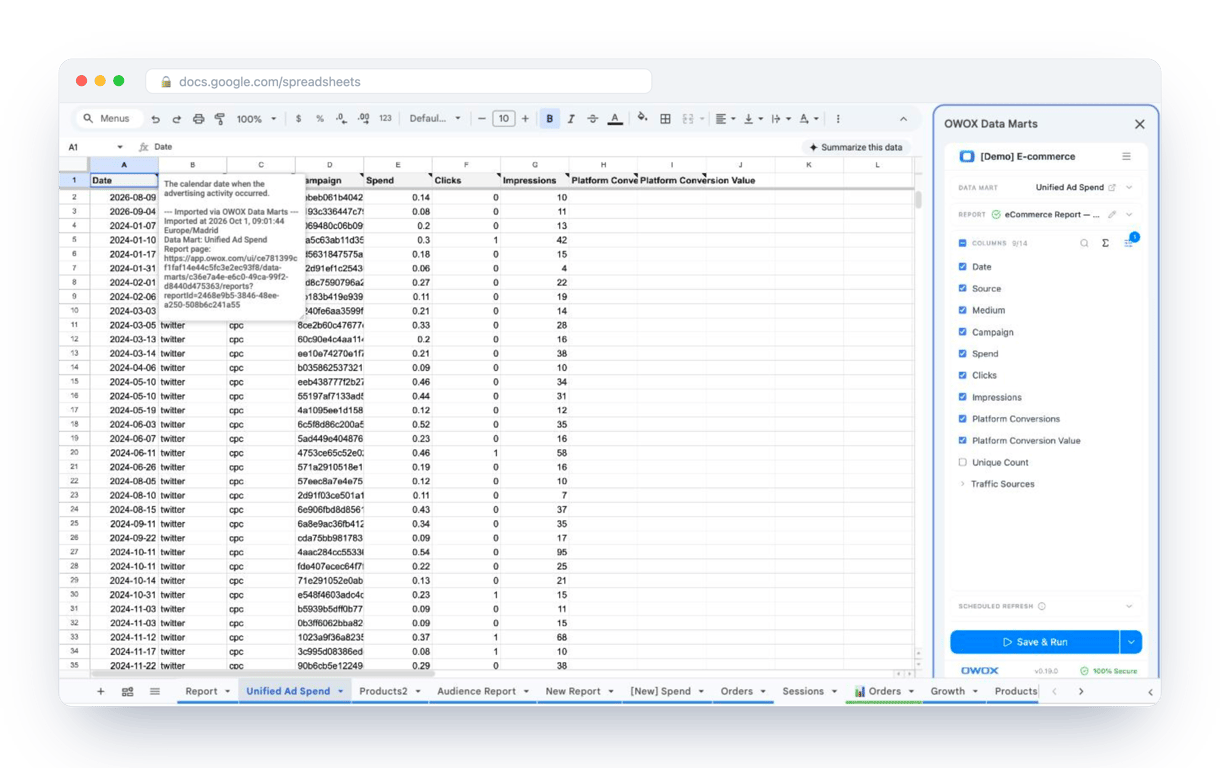
The OWOX Data Marts extension for Google Sheets covers that half. A data analyst publishes a data mart (a table or an SQL query in your data warehouse) and makes it available for reports. In Sheets you open the extension, pick the data mart, tick the columns you want and run it. The rows land in a tab, ready for your formulas.
What changes for the person who maintains the sheet:
- Refresh replaces re-export. Refresh current report in the extension menu re-runs the same pull, and a scheduled refresh keeps the tab current without anyone touching it.
- The source is written on the sheet. The header cell of an imported tab carries a note with the data mart it came from, the time of the import and a link to the report.
- No SQL and no warehouse access needed. The analyst decides which data marts and columns are available. You choose from that list.
The extension does not write or change the analyst’s SQL. When the two tables are joined once in that SQL, the sheet receives the attributes next to the keys, and the lookup is no longer needed. The extension comes with the OWOX Cloud plans of OWOX Data Marts; spreadsheet reporting describes both ways data reaches a sheet.
Turn your data into decisions.
Governed data marts give you the clean foundation ML needs to actually work.
- No AI hallucinations
- Analyst-governed definitions
- Every number traces to SQL
Frequently Asked Questions
What are some tips while handling HLOOKUP Function in Google Sheets?
When using HLOOKUP, ensure your search_key is in the first row of the range. Use an accurate index to retrieve the correct row. Set [is_sorted] to FALSE for exact matches. Combine with IFERROR to handle errors gracefully, and use named ranges for clarity.
What is the syntax of HLOOKUP?
The syntax of HLOOKUP in Google Sheets is =HLOOKUP(search_key, range, index, [is_sorted]). Here, search_key is the value to search for, range is the table array, index is the row number to return from, and [is_sorted] is optional, indicating whether the data is sorted.
What is the #VALUE! Error in HLOOKUP?
HLOOKUP returns #VALUE! when the index is 0 or negative: rows are counted from 1. An index larger than the number of rows in the range returns #REF!, and a key that is not in the first row returns #N/A.
How can you combine VLOOKUP with HLOOKUP?
The usual reason to combine them is a two-way lookup: find a cell by a column key and a row label. Use MATCH for the row number inside HLOOKUP, for example HLOOKUP("A003", C2:G5, MATCH("Stock", B2:B5, 0), FALSE), or INDEX with two MATCH functions: INDEX(C3:G5, MATCH("Stock", B3:B5, 0), MATCH("A003", C2:G2, 0)).
What is the Difference Between HLOOKUP and VLOOKUP?
HLOOKUP searches for a value horizontally across the top row of a range and returns a value from a specified row. VLOOKUP, on the other hand, searches vertically down the first column and returns a value from a specified column. Both functions help find data, but in different orientations.
How Do I Use HLOOKUP in Google Sheets?
To use HLOOKUP in Google Sheets, input =HLOOKUP(search_key, range, index, [is_sorted]). This function searches for a key in the first row of a range and returns a value from a specified row. Ensure the index corresponds to the row you want to retrieve data from within the range.