COUNTIF and COUNTIFS in Google Sheets: criteria and examples
COUNTIF counts the cells in a range that meet one condition; COUNTIFS counts the rows that meet several at once. This guide lists the criteria for text, numbers, dates, wildcards and blanks, shows OR logic without double counting, counting across sheets, COUNTIF in conditional formatting, and the mistakes that return a wrong number without an error.

COUNTIF counts the cells in a range that meet one condition:
=COUNTIF(C3:C9, "Available")
COUNTIFS counts the rows that meet several conditions at the same time:
=COUNTIFS(C3:C9, "Available", D3:D9, ">400")
The condition (the criterion) is where most mistakes happen. This table covers the forms you will need:
| To count cells that | Criterion | Example |
|---|---|---|
| Equal a text | "Available" |
=COUNTIF(C3:C9, "Available") |
| Equal a number | 500 |
=COUNTIF(D3:D9, 500) |
| Are greater or less than a number | ">500", "<=500" |
=COUNTIF(D3:D9, ">500") |
| Are not equal to a value | "<>East" |
=COUNTIF(D3:D9, "<>East") |
| Compare with a value in another cell | ">"&F3 |
=COUNTIF(D3:D9, ">"&F3) |
| Start with, end with or contain a text | "James*", "*Rep", "*Account*" |
=COUNTIF(B3:B9, "James*") |
| Match a pattern with one unknown character | "?est" |
=COUNTIF(D3:D9, "?est") |
| Hold a date | DATE(2024,4,9) |
=COUNTIF(C3:C9, DATE(2024,4,9)) |
| Hold a date on or after a day | ">="&DATE(2024,4,1) |
=COUNTIF(C3:C9, ">="&DATE(2024,4,1)) |
| Are checked checkboxes | TRUE |
=COUNTIF(C3:C9, TRUE) |
| Are empty | "" |
=COUNTIF(D3:D9, "") |
| Are not empty | "<>" |
=COUNTIF(D3:D9, "<>") |
| Hold any text | "*" |
=COUNTIF(B3:D9, "*") |
Text criteria are not case-sensitive: “available” and “Available” are counted together.
COUNTIF syntax
=COUNTIF(range, criterion)
- range: the cells to check.
- criterion: the condition. A number, a text or an expression in quotes, or a reference to a cell that holds the value.
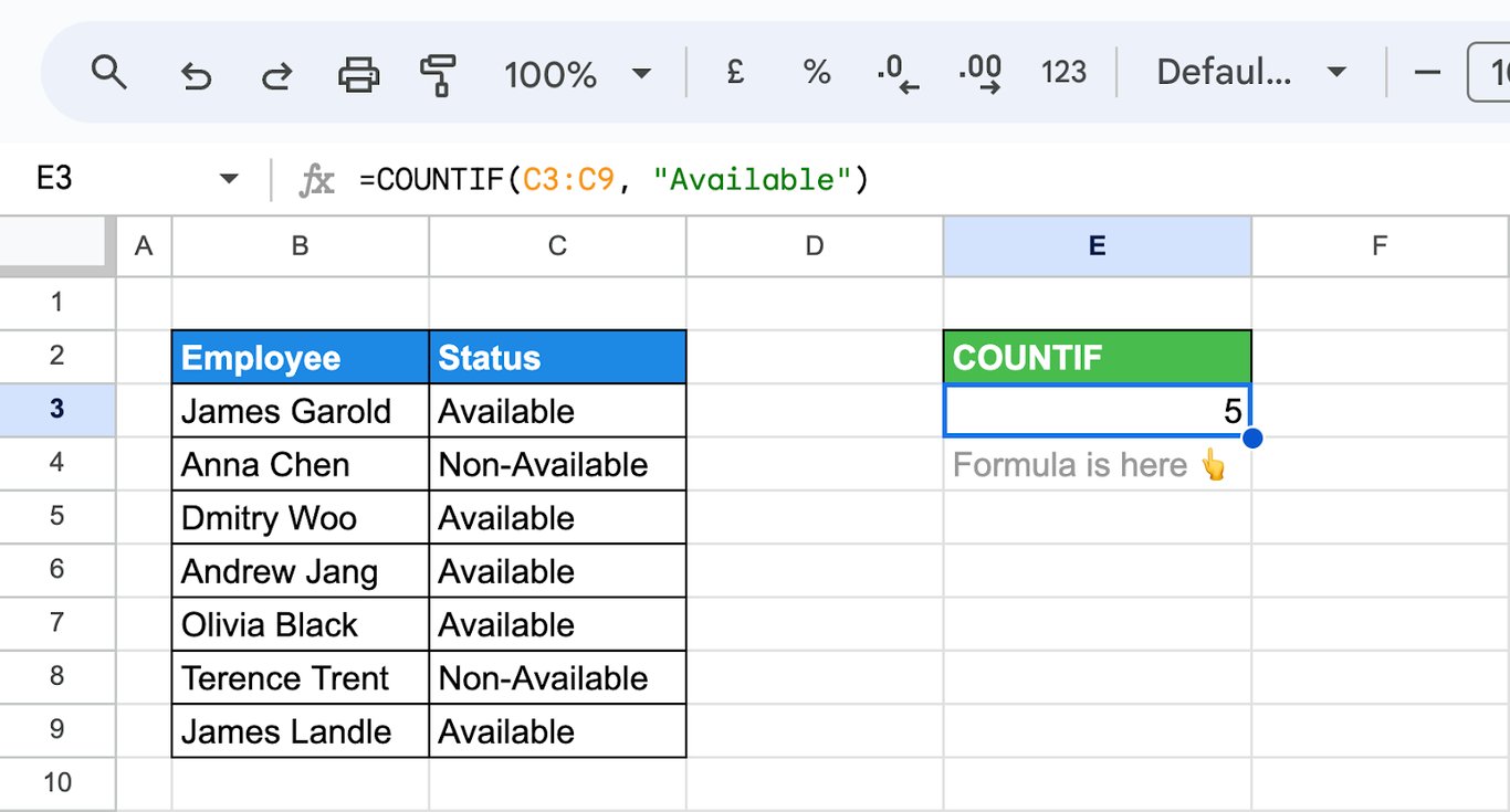
Five of the seven employees have the status “Available”. The match is on the whole cell: “Non-Available” is not counted, because the criterion has no wildcards.
COUNTIFS syntax
=COUNTIFS(criteria_range1, criterion1, [criteria_range2, criterion2, ...])
Each range is followed by its own criterion. A row is counted only when all conditions are true for it (AND logic), and all ranges must have the same number of rows.
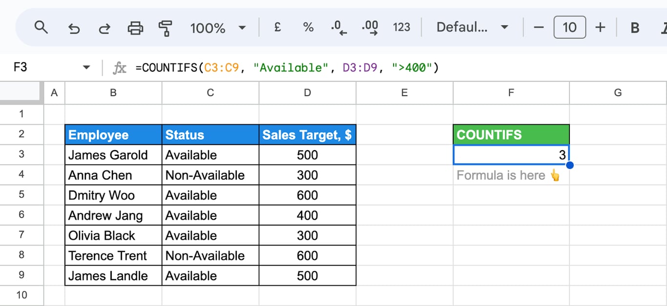
Three employees are available and have a sales target above 400.
To count for several values at once, there is no need to copy the formula row by row. Put the values in a column and let ARRAYFORMULA fill the counts: =ARRAYFORMULA(COUNTIF(C3:C9, F3:F5)). COUNTIFS does not expand this way; the guide to array formulas explains which functions do.
OWOX Data Marts
See your first report built in real time. 15 minutes.
- Connect your data warehouse
- Pick your metrics
- Get a live Google Sheets report
In the time it takes to write a ticket. Then imagine never writing that ticket again.
Book a DemoWe'll use your actual use case
Criteria in practice
Text and numbers in a cell
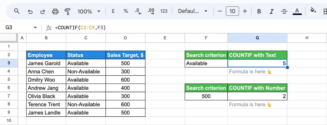
Keep the criterion in a cell and the formula does not have to be edited when the question changes:
=COUNTIF(C3:C9, F3)
The same works for a number:
=COUNTIF(D3:D9, F7)
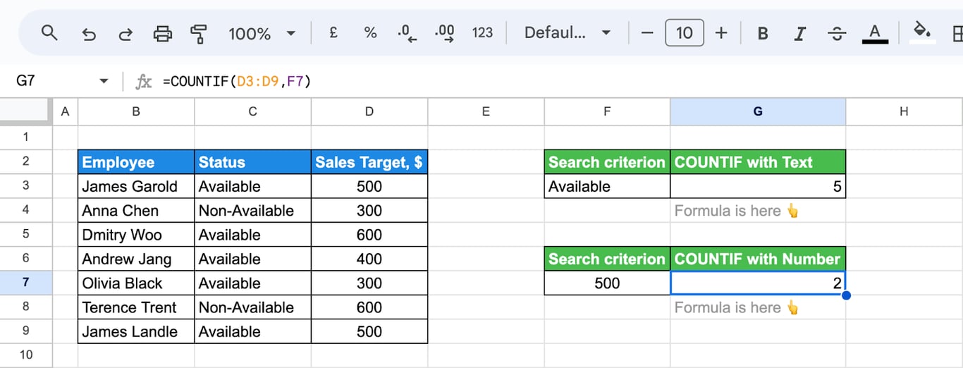
To compare with the cell instead of matching it, join the operator and the reference with an ampersand: =COUNTIF(D3:D9, ">"&F7). Writing ">F7" inside the quotes looks for the text “>F7”.
Greater than, less than, not equal
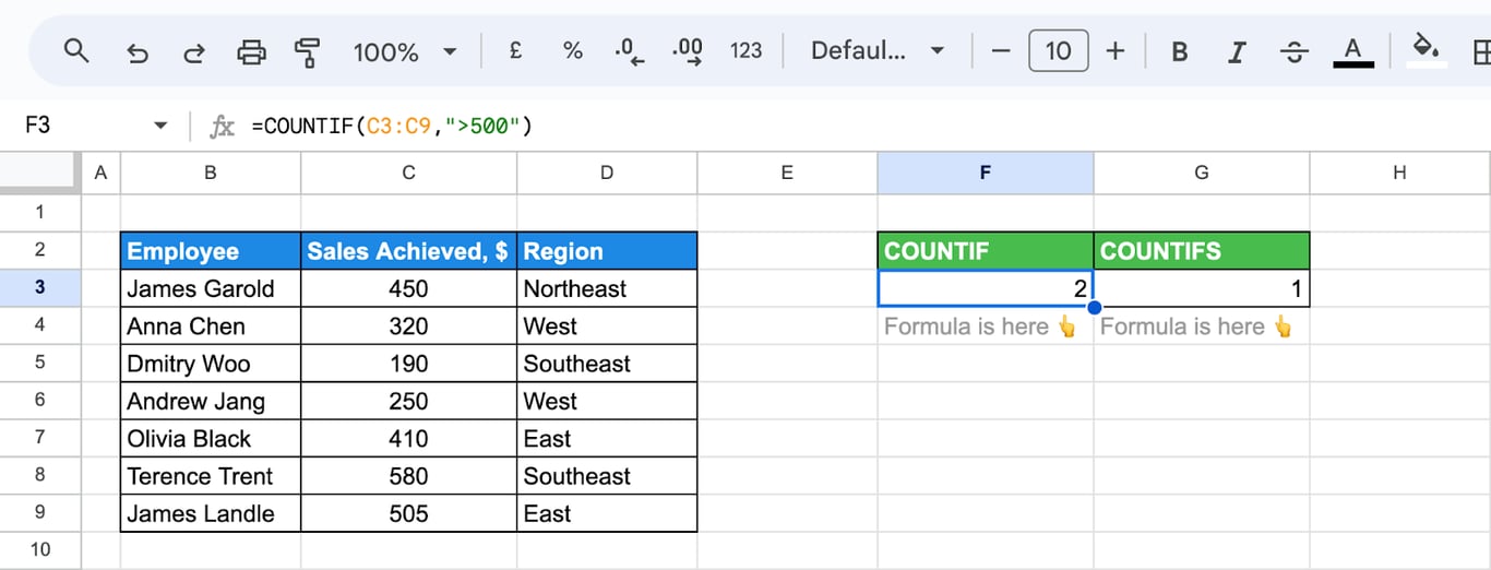
The operator and the number go together in one pair of quotes:
=COUNTIF(C3:C9, ">500")
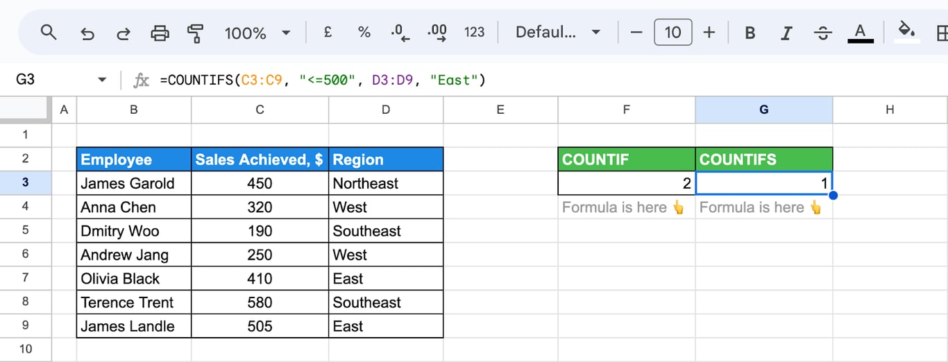
With COUNTIFS, a comparison can be combined with a text condition:
=COUNTIFS(C3:C9, "<=500", D3:D9, "East")
Between two numbers
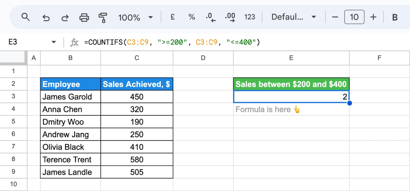
Use the same range twice, once for each limit:
=COUNTIFS(C3:C9, ">=200", C3:C9, "<=400")
Wildcards
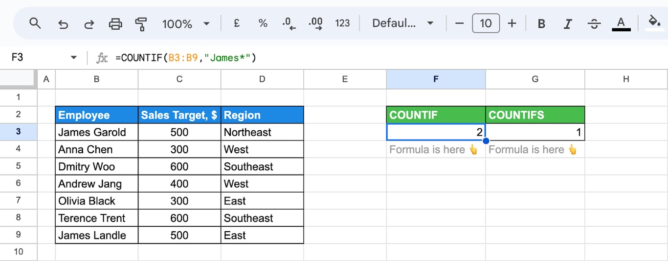
An asterisk stands for any number of characters, a question mark for exactly one.
=COUNTIF(B3:B9, "James*")
=COUNTIFS(D3:D9, "?est", C3:C9, "300")
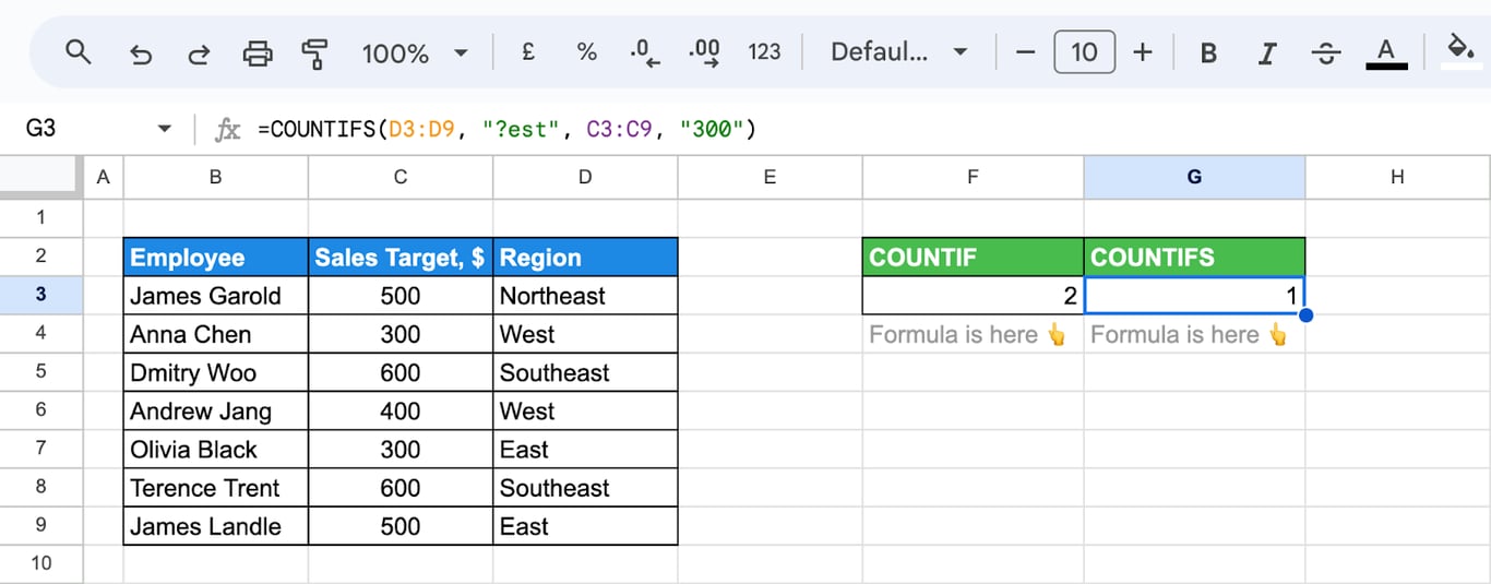
“?est” matches “West” and would match “Test”, but not “East” or “Northeast”. Two limits to remember:
- Wildcards work on text only.
=COUNTIF(D3:D9, "*5*")returns 0 on a column of numbers, even if every number contains a 5. - To count cells that contain a real asterisk or question mark, put a tilde in front:
"~*".
Dates
A date typed as text in the criterion is read in the format of the spreadsheet’s locale. The example sheet uses the day/month/year order, so “9/4/2024” is 9 April:
=COUNTIF(C3:C9, "9/4/2024")
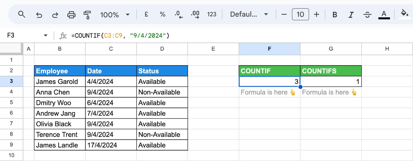
In a sheet with a United States locale the same formula would look for 4 September. A formula that survives a change of locale builds the date with DATE:
=COUNTIF(C3:C9, DATE(2024,4,9))
For a period, use COUNTIFS with two limits on the same column:
=COUNTIFS(C3:C9, ">="&DATE(2024,4,1), C3:C9, "<"&DATE(2024,5,1))
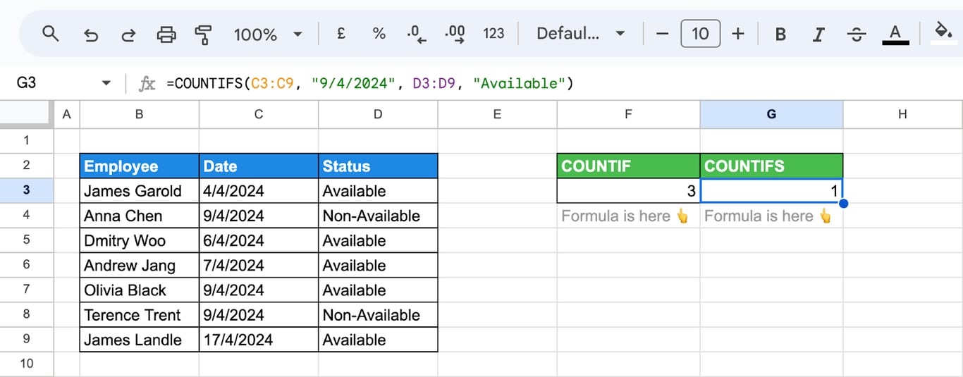
A date condition combines with any other:
=COUNTIFS(C3:C9, "9/4/2024", D3:D9, "Available")
More on how Sheets stores dates in the guide to dates and times.
Checkboxes
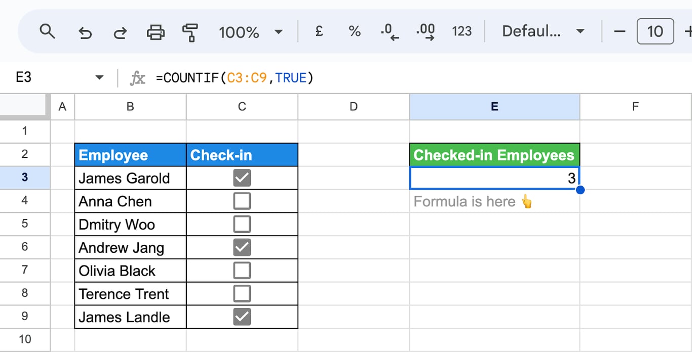
A checked box holds TRUE, an unchecked one FALSE:
=COUNTIF(C3:C9, TRUE)
Blank and non-blank cells
=COUNTIF(D3:D9, "<>")
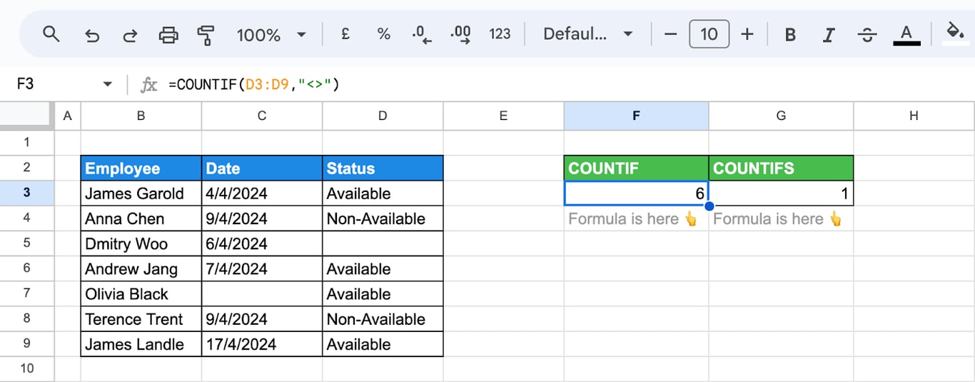
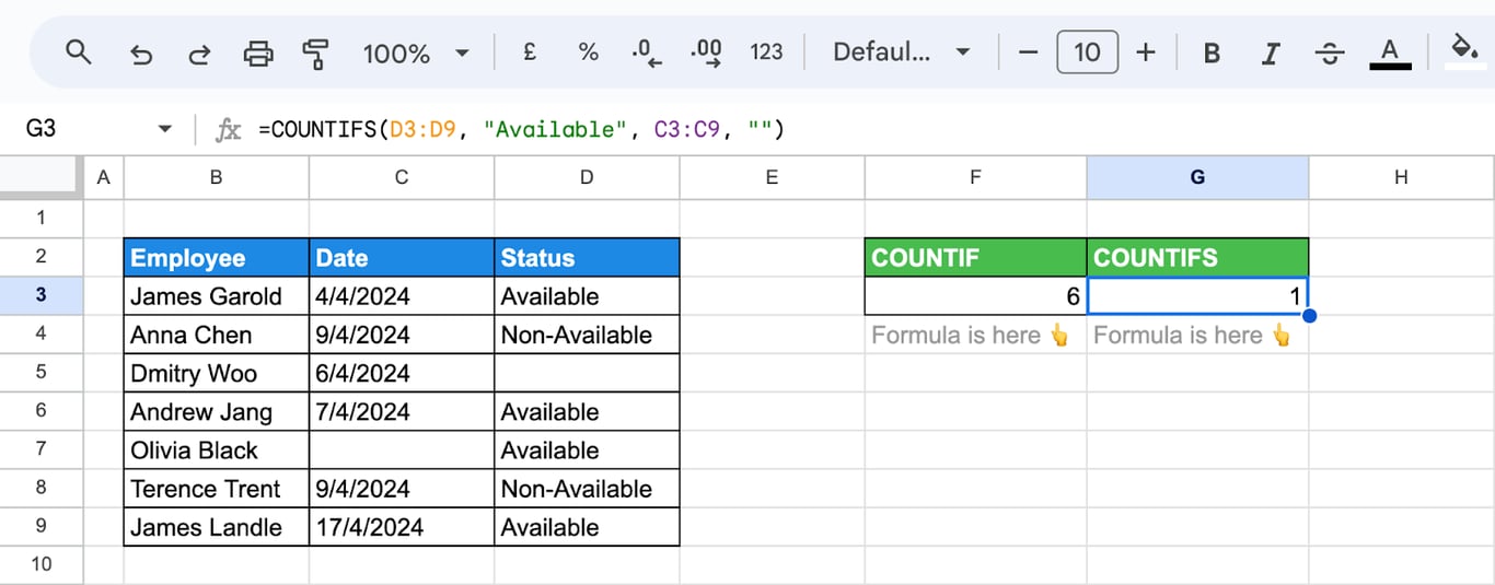
“<>” counts the cells that are not empty, "" the cells that are. In COUNTIFS the empty criterion finds incomplete rows, for example available employees with no date:
=COUNTIFS(D3:D9, "Available", C3:C9, "")
For blanks alone there is a function of its own:
=COUNTBLANK(B3:B9)
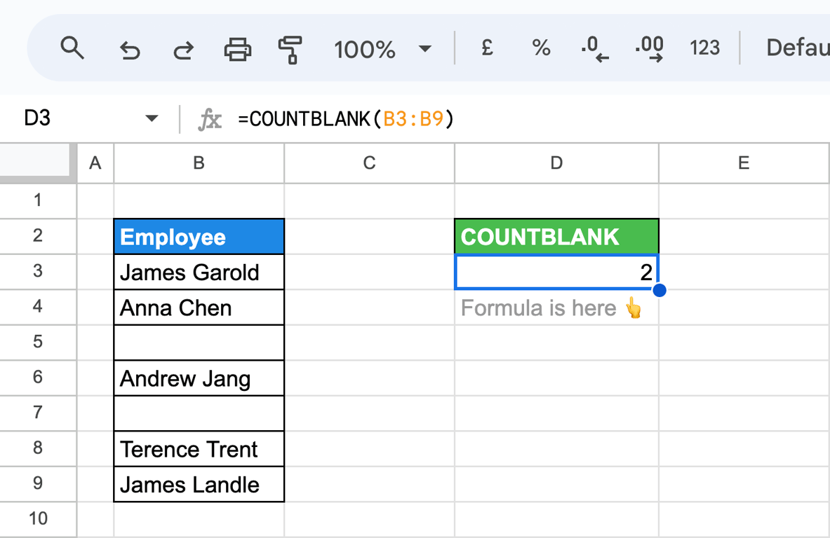
COUNTBLANK takes several ranges, =COUNTBLANK(B3:B9, D3:D9), and counts cells with a formula that returns an empty text as blank. COUNT and COUNTA cover the opposite case.
COUNTIF with multiple criteria: AND and OR
COUNTIF with multiple criteria: AND and OR
AND (all conditions true for the same row) is what COUNTIFS does.
OR (any of the conditions) needs more care. Adding two COUNTIF results works only when a cell cannot match both conditions:
=COUNTIF(C3:C9, "*Manager*") + COUNTIF(C3:C9, "*Account*")
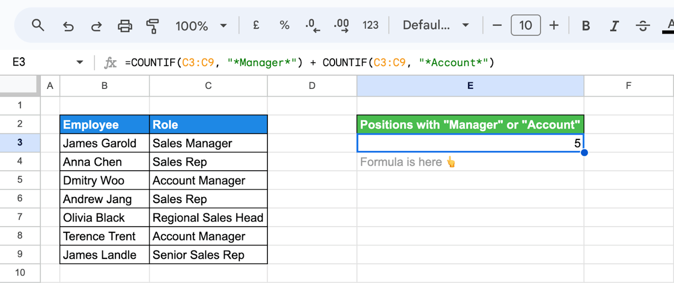
The formula returns 5, but only three rows contain “Manager” or “Account”. The two Account Managers are counted twice, once by each COUNTIF. To count each row once, test the condition row by row:
=SUMPRODUCT(REGEXMATCH(C3:C9, "Manager|Account"))
REGEXMATCH returns TRUE for a row that contains either word, and SUMPRODUCT adds the TRUE values up. Unlike COUNTIF, REGEXMATCH is case-sensitive.
When the alternatives are whole values and exclude each other, a list in curly braces is shorter:
=ARRAYFORMULA(SUM(COUNTIFS(C3:C9, {"Sales Rep","Account Manager"})))
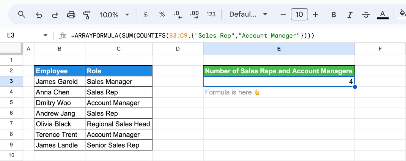
ARRAYFORMULA is required here. Without it the formula counts only the first value of the list and returns a smaller number, with no error.
Count unique values
COUNTUNIQUE counts how many different values a range holds:
=COUNTUNIQUE(C3:C9)
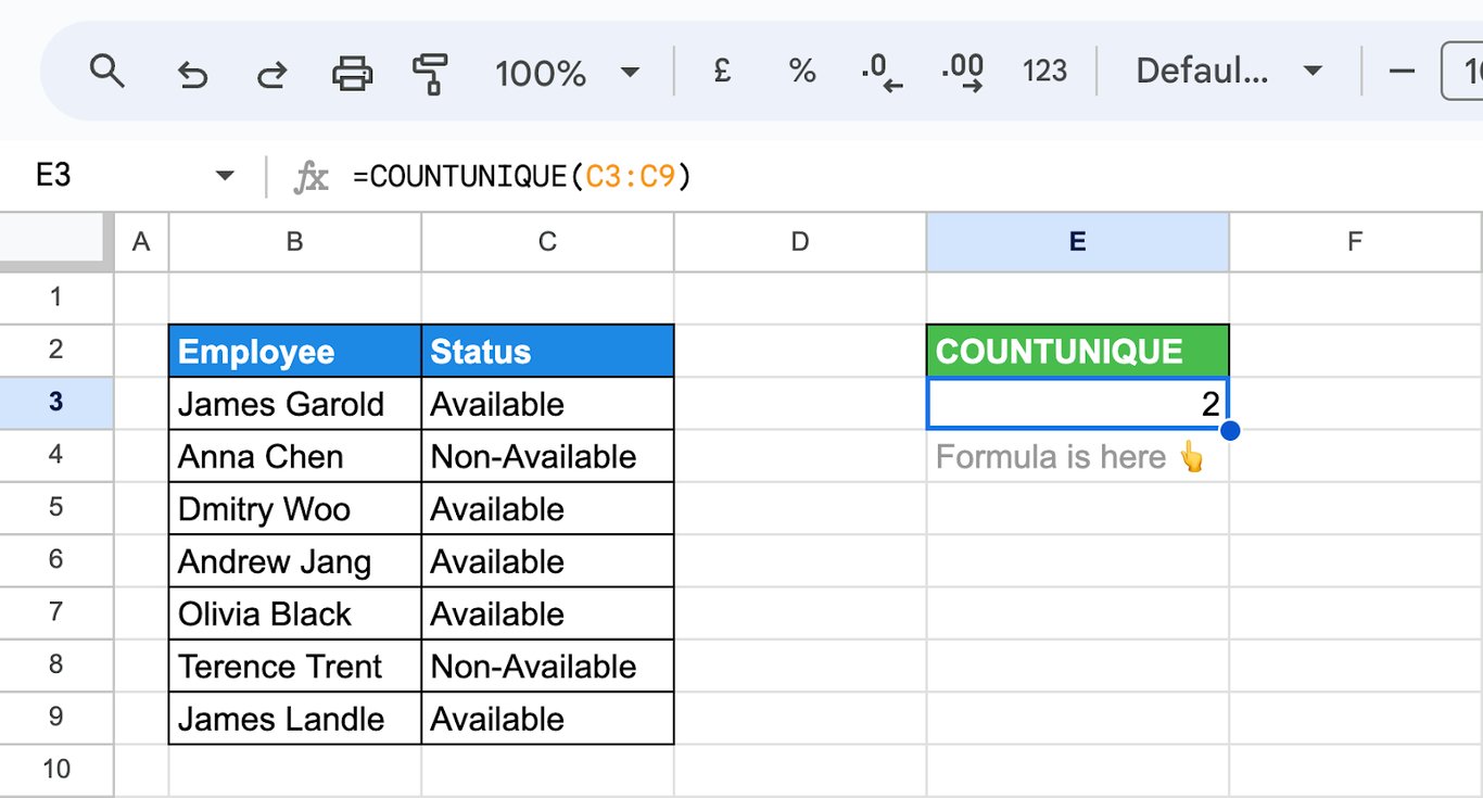
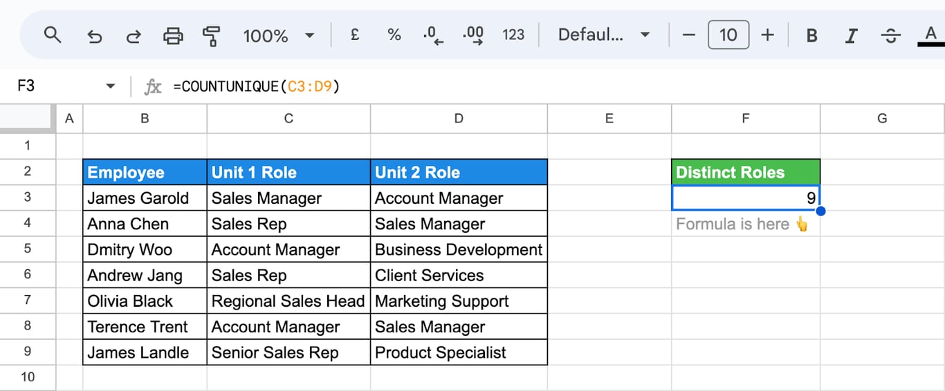
The range can span several columns:
=COUNTUNIQUE(C3:D9)
COUNTUNIQUEIFS adds conditions. Its first argument is the range to count unique values in, followed by pairs of range and criterion:
=COUNTUNIQUEIFS(B3:B9, C3:C9, "Available", D3:D9, ">=500")
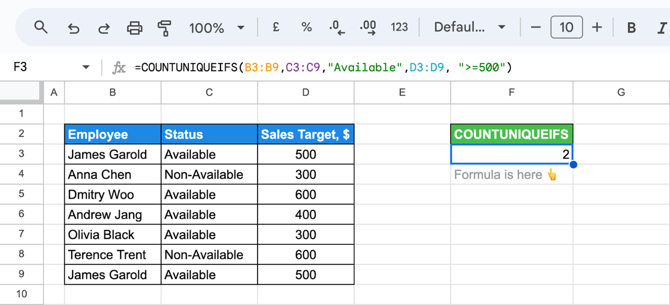
James Garold appears twice with the status “Available” and a target of 500, and is counted once: the result is 2 employees, not 3 rows.
=COUNTUNIQUEIFS(C3:C9, D3:D9, ">=200", D3:D9, "<=400")
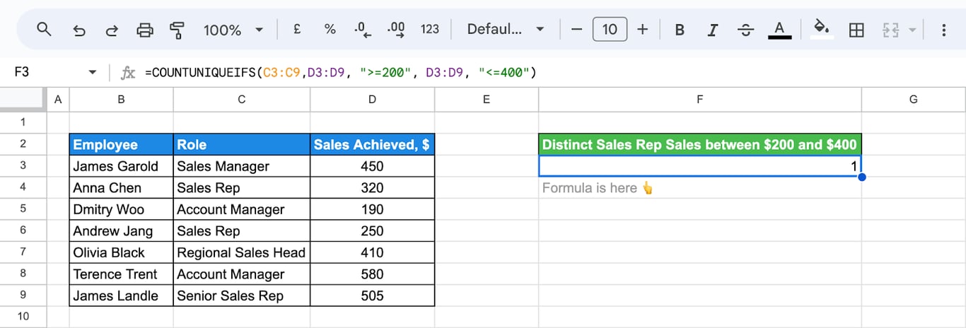
Two sales reps have sales between 200 and 400, and both hold the same role, so the number of distinct roles is 1.
A quick test for duplicates compares the number of unique values with the number of filled cells:
=IF(COUNTUNIQUE(C3:C9)=COUNTA(C3:C9), "No Duplicates", "Duplicates Found")
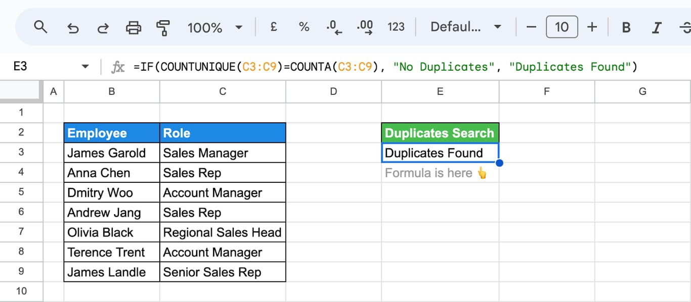
To see the values themselves, use UNIQUE.
COUNTIF and COUNTIFS across sheets
COUNTIF and COUNTIFS across sheets
To count in another sheet, put the sheet name and an exclamation mark before the range. A name with spaces goes in single quotes:
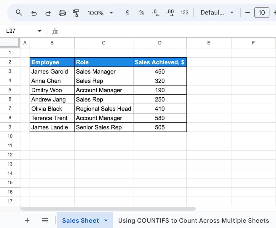
=COUNTIFS('Sales Sheet'!C3:C9, "Sales Rep", 'Sales Sheet'!D3:D9, ">300")
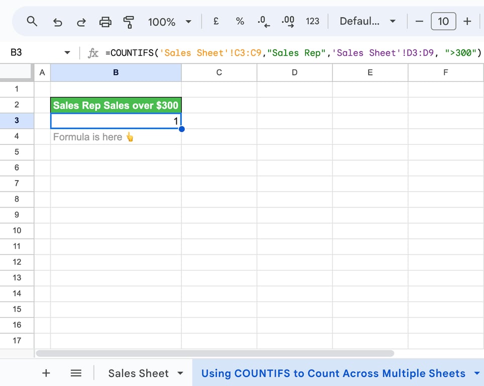
To count over several sheets at once, add one COUNTIF for each sheet:
=COUNTIF(January!C3:C9, "Sales Rep") + COUNTIF(February!C3:C9, "Sales Rep")
or stack the ranges into one with curly braces and a semicolon:
=COUNTIF({January!C3:C9; February!C3:C9}, "Sales Rep")
For another spreadsheet file, bring the range in with IMPORTRANGE first.
COUNTIF in conditional formatting
COUNTIF in conditional formatting
COUNTIF is the usual way to highlight duplicates:
- Select the range, here C3:C9.
- Click Format > Conditional formatting.
- Under Format cells if, choose Custom formula is.
- Enter the formula and pick a fill color.
=COUNTIF($C$3:$C$9, C3)>1
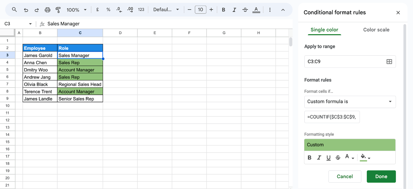
The range inside COUNTIF is locked with dollar signs; the criterion C3 is not, and must point to the first cell of the selected range. Sheets then shifts it down row by row.
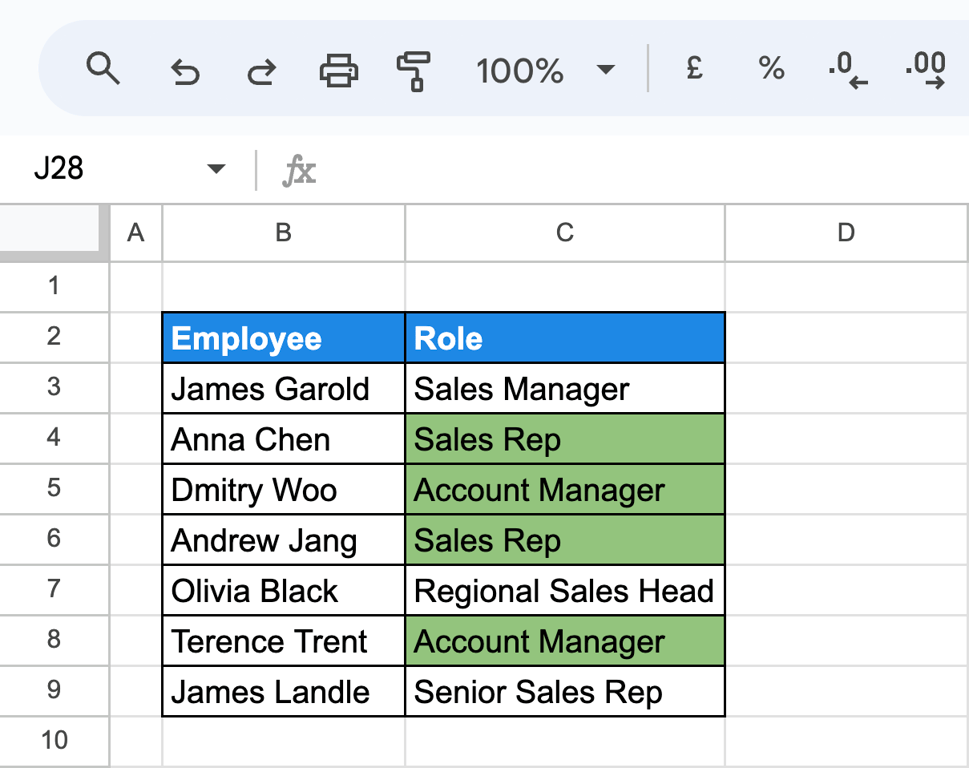
COUNTIF cannot work the other way round: no built-in function counts cells by their fill color. Count by the rule that colored them. If the Account Manager cells are yellow because of a rule, count the Account Managers.
COUNTIF with other functions
VLOOKUP: count by a value that has to be looked up first
The attendance table holds employee IDs, the search cell a name. VLOOKUP finds the ID and COUNTIF counts it:
=COUNTIF(B12:F15, VLOOKUP(F2, B3:C9, 2, FALSE))
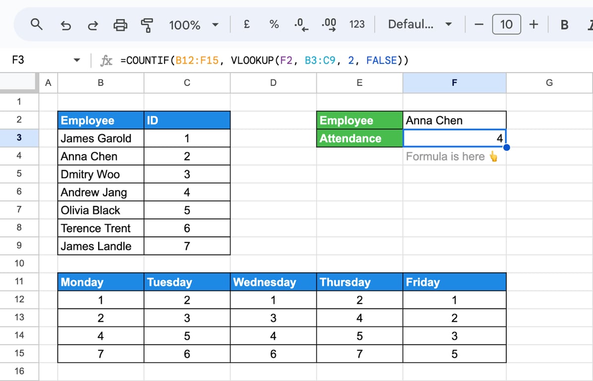
AVERAGE: count the values above the average
=COUNTIF(D3:D9, ">"&AVERAGE(D3:D9))
Any function that returns one value can be joined to the operator this way.
QUERY: counts for every group at once
COUNTIFS answers one question with one number:
=COUNTIFS(C3:C9, "Sales Rep", D3:D9, "Available", E3:E9, ">200")
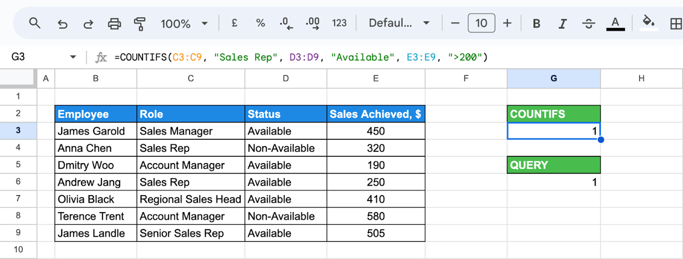
The same count with QUERY:
=QUERY(C3:E9, "SELECT COUNT(C) WHERE C = 'Sales Rep' AND D = 'Available' AND E > 200 LABEL COUNT(C) ''")
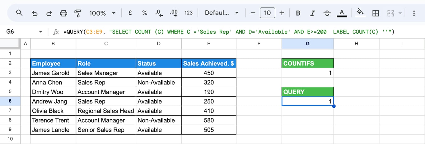
For a single number COUNTIFS is shorter. QUERY is worth it when you need the count for every role in one formula: "SELECT C, COUNT(C) GROUP BY C" returns a small table that grows when a new role appears. Text in a QUERY condition is case-sensitive, in COUNTIFS it is not.
Errors and wrong results
⚠️ Error: #VALUE! in COUNTIFS.
✅ Solution: The ranges have different sizes, for example C3:C12 and D3:D11. Make them the same height.
⚠️ Error: #N/A in COUNTIFS.
✅ Solution: A range has no criterion. The arguments come in pairs.
⚠️ Error: The result is 0, although the value is in the range.
✅ Solution: Check four things. A text criterion without quotes, =COUNTIF(C3:C9, Available), returns 0 without an error. A space at the end of the cells prevents an exact match: clean them with TRIM or use "Available*". Numbers stored as text are not counted by ">500". A wildcard does not match numbers.
⚠️ Error: The result is too high.
✅ Solution: Two COUNTIF results were added and some cells match both conditions, or a wildcard matches more than intended: "*Rep*" also counts “Reporting”.
⚠️ Error: The date criterion finds nothing or the wrong day.
✅ Solution: The date text is read in the locale of the spreadsheet. Use DATE(year, month, day).
⚠️ Error: ">F3" does not compare with cell F3.
✅ Solution: The reference must be outside the quotes: ">"&F3.
⚠️ Error: A formula parse error.
✅ Solution: In locales that use a comma as the decimal separator, the arguments are separated with semicolons: =COUNTIF(C3:C9; "Available").
⚠️ Error: Upper and lower case are counted together.
✅ Solution: COUNTIF ignores case. For a case-sensitive count use =SUMPRODUCT(EXACT(C3:C9, "Available")); see the guide to EXACT.
Related Google Sheets functions
Related Google Sheets functions
- COUNT and COUNTA: Count numbers and non-empty cells.
- SUMIF and SUMIFS: Add up the values that meet the conditions.
- AVERAGEIF: Average the values that meet a condition.
- FILTER: Return the matching rows instead of counting them.
- UNIQUE: List the distinct values.
- QUERY: Count, sum and group in one formula.
- Pivot tables: Counts for every category without formulas.
- IF and IFS: Return a value depending on a condition.
- Data validation: Keep the values you count consistent.
A count is only as good as the rows under it
A count is only as good as the rows under it
COUNTIFS gives an exact answer about the rows in the sheet. Whether those rows are complete is a different question: an export pasted last Tuesday is counted as carefully as fresh data, and two people counting “available reps” on two copies of the table get two numbers. The formula cannot see that.
The OWOX Data Marts extension for Google Sheets covers that half. A data analyst publishes a data mart (a table or an SQL query in your data warehouse) and makes it available for reports. In Sheets you open the extension, pick the data mart, tick the columns you want and run it. The rows land in a tab, ready for your formulas.
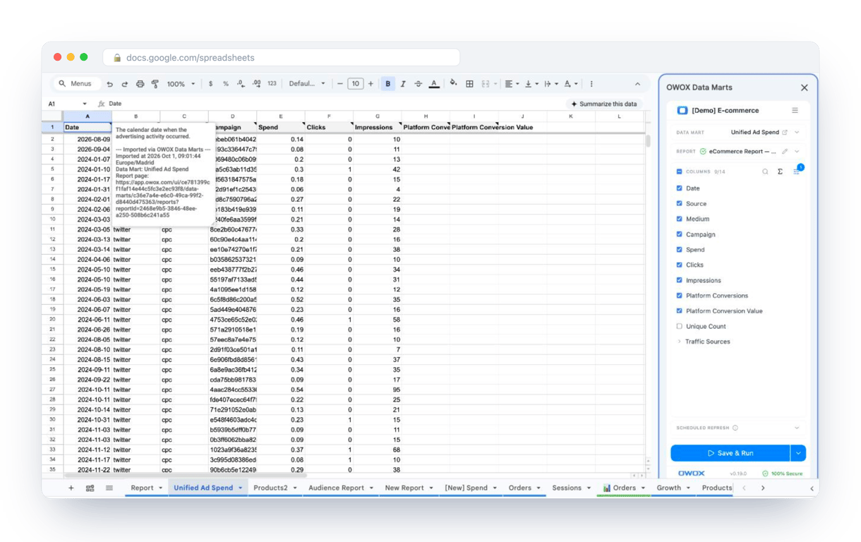
What changes for the person who maintains the sheet:
- Refresh replaces re-export. Refresh current report in the extension menu re-runs the same pull, and a scheduled refresh keeps the tab current without anyone touching it.
- The source is written on the sheet. The header cell of an imported tab carries a note with the data mart it came from, the time of the import and a link to the report.
- No SQL and no warehouse access needed. The analyst decides which data marts and columns are available. You choose from that list.
The extension does not write or change the analyst’s SQL. COUNTIF and COUNTIFS then run on the same refreshed rows for everyone who opens the report. The extension comes with the OWOX Cloud plans of OWOX Data Marts; spreadsheet reporting describes both ways data reaches a sheet.
Turn your data into decisions.
Governed data marts give you the clean foundation ML needs to actually work.
- No AI hallucinations
- Analyst-governed definitions
- Every number traces to SQL
Frequently Asked Questions
What are some common errors when using COUNTIF and COUNTIFS in Google Sheets, and how can I fix them?
COUNTIFS returns #VALUE! when its ranges have different sizes and #N/A when a range has no criterion. The mistakes that give a wrong number without an error are harder to spot: a text criterion without quotes returns 0, a comparison with a cell must be written as ">"&F3 with the reference outside the quotes, wildcards do not match numbers, and a date typed as text is read in the spreadsheet's locale, so build it with DATE.
What are some best practices for using COUNTIF and COUNTIFS in Google Sheets?
Consistent Criteria Format: Ensure criteria are consistent (">10" instead of "> 10"). Range Size Consistency: Use ranges of equal size in COUNTIFS to avoid errors.Named Ranges: Utilize named ranges for clarity (=COUNTIF(Apples, ">10")).Regular Testing: Test formulas with sample data to verify accuracy.
How do I use COUNTIFS to count cells with multiple criteria in Google Sheets?
COUNTIFS counts cells meeting multiple criteria: COUNTIFS(range1, criterion1, range2, criterion2, ...). Example: COUNTIFS(A1:A10, ">10", B1:B10, "<>0") counts cells >10 in A1 and not 0 in B1.
How can I count unique values with multiple criteria using COUNTIF in Google Sheets?
Use COUNTUNIQUEIFS. Its first argument is the range to count unique values in, followed by pairs of range and criterion: COUNTUNIQUEIFS(B3:B9, C3:C9, "Available", D3:D9, ">=500") counts each employee once, however many rows they have with the status Available and a target of at least 500.
What is the syntax of the COUNTIF function in Google Sheets?
The syntax of COUNTIF in Google Sheets is COUNTIF(range, criterion). Specify range as the cells to evaluate and criterion as the condition or pattern to count. Example: COUNTIF(A1:A10, ">10") counts cells in A1 greater than 10.
How can I count cells with specific text using COUNTIF in Google Sheets?
To count cells with specific text, use COUNTIF(range, "text"). Example: COUNTIF(A1:A10, "apple") counts cells in A1 containing "apple". Use wildcards like * for partial matches (COUNTIF(A1:A10, "*apple*")).