LOOKUP function in Google Sheets: syntax, examples and when to use another lookup
LOOKUP finds a value in a sorted row or column and returns the value in the same position of another range. It never asks for an exact match, so on unsorted data it returns wrong values without an error. This guide covers the syntax, examples, the sorting rule, and the cases where VLOOKUP, XLOOKUP or INDEX with MATCH are the safer choice.

The LOOKUP function searches one row or column for a value and returns the value in the same position of another row or column:
=LOOKUP(H3, B3:B12, D3:D12)
The formula looks for the value of H3 in B3:B12 and returns the matching cell of D3:D12.
One rule decides whether the result can be trusted: the search range has to be sorted in ascending order. LOOKUP has no exact-match setting. It assumes sorted data, and when it does not find the key, it returns the nearest smaller value. On an unsorted range it returns a wrong value with no error.
| LOOKUP | VLOOKUP | XLOOKUP | |
|---|---|---|---|
| Exact match on unsorted data | No | Yes, with FALSE | Yes, by default |
| Searches a row or a column | Both | Columns only | Both |
| Result can be left of the key | Yes | No | Yes |
| Key not found | Nearest smaller value, or #N/A if there is none | #N/A | #N/A, or a text you choose |
Use LOOKUP for what it is good at: finding the band a number falls into, such as a price tier or a grade. For lookups by ID or name, VLOOKUP with FALSE or XLOOKUP is the safer choice.
LOOKUP syntax
LOOKUP has two forms.
With a search range and a result range:
=LOOKUP(search_key, search_range, result_range)
- search_key: the value to look for: a number, a text or a cell reference.
- search_range: one row or one column to search, sorted in ascending order.
- result_range: one row or one column to return the value from. It has to be the same size as the search range.
With one array:
=LOOKUP(search_key, search_result_array)
- search_result_array: a range with several columns or rows. LOOKUP searches its first column and returns the value from its last column. If the range is wider than it is tall, it searches the first row and returns from the last row.
Example with two ranges
The table lists laptops with an item ID, brand, model, price and quantity, sorted by ID. To return the model for the ID typed in H3:
=LOOKUP(H3, B3:B12, D3:D12)
- H3: the item ID to look for, LT009.
- B3:B12: the item IDs, in ascending order.
- D3:D12: the models.
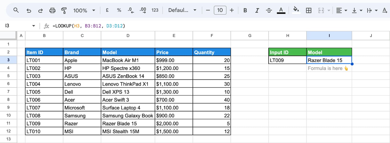
The formula returns Razer Blade 15.
Example with one array
The same lookup with the single-array form:
=LOOKUP(H3, B3:D12)
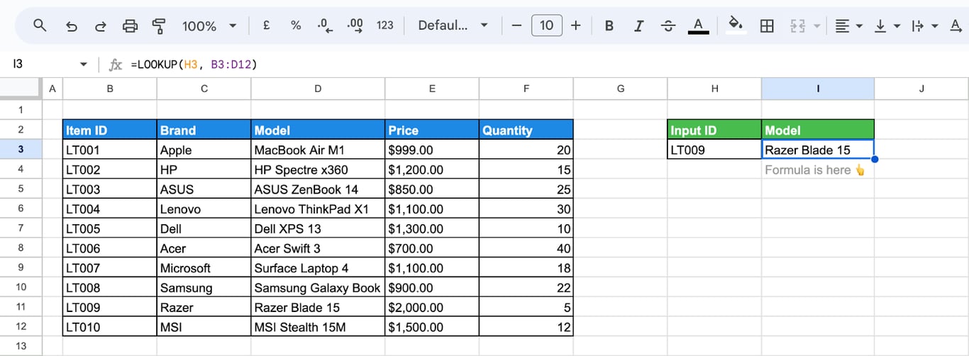
LOOKUP searches column B, the first column of the range, and returns the value from column D, the last one. To return a different column, change where the range ends.
Why the search range must be sorted
Why the search range must be sorted
Here the same table is shuffled, and the formula is unchanged:
=LOOKUP(H3, B3:B12, D3:D12)
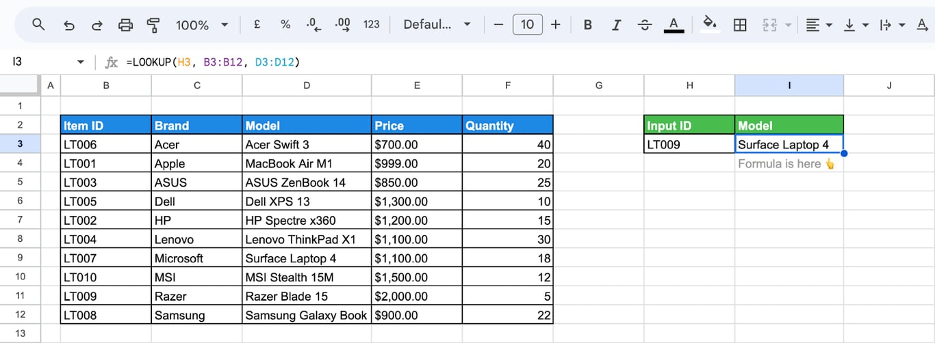
The ID LT009 is in the table, yet LOOKUP returns Surface Laptop 4, the model of another row. There is no error message. LOOKUP searches by halving the range again and again, which is fast but only works when the values are in order.
After sorting the table by item ID, the same formula returns the right model.
Sorting matters for a second reason: what happens when the key is not in the range. LOOKUP then returns the last value that is smaller than the key. With thresholds of 1500, 1800 and 2100, =LOOKUP(2000, {1500; 1800; 2100}, {"a"; "b"; "c"}) returns “b”, the band that starts at 1800. A key below the smallest value, 1000 here, returns #N/A.
That behaviour is exactly what a tier table needs. With the lower limit of each discount band in one column and the discount in the next, =LOOKUP(order_amount, limits, discounts) returns the discount for any amount.
OWOX Data Marts
See your first report built in real time. 15 minutes.
- Connect your data warehouse
- Pick your metrics
- Get a live Google Sheets report
In the time it takes to write a ticket. Then imagine never writing that ticket again.
Book a DemoWe'll use your actual use case
More examples of LOOKUP
Return a text value
To return the brand for an item ID:
=LOOKUP(H3, B3:B12, C3:C12)
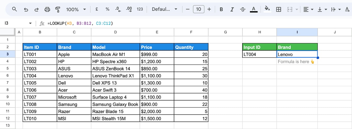
The formula returns Lenovo, the brand of LT004.
Return a number
To return the price:
=LOOKUP(H3, B3:B12, E3:E12)
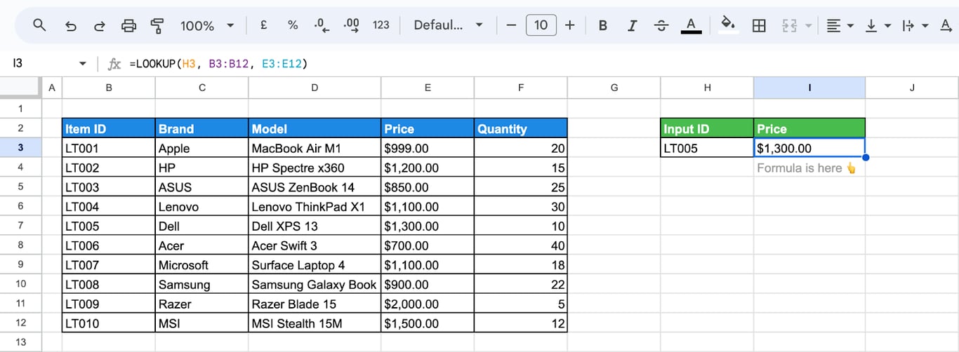
The formula returns $1,300.00, the price of LT005. The result keeps its type, so it can be used in further calculations.
Search a row
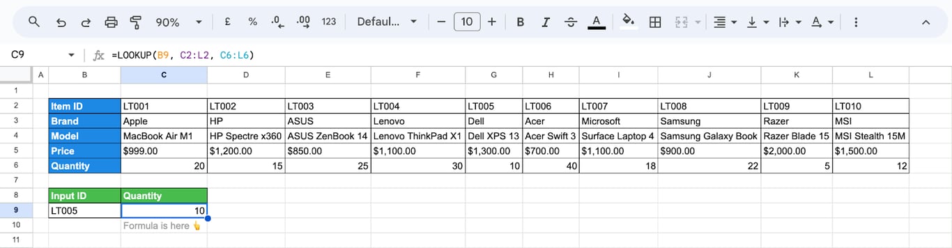
LOOKUP works the same way on a table laid out sideways. With the item IDs in row 2 and the quantities in row 6:
=LOOKUP(B9, C2:L2, C6:L6)
- B9: the item ID to look for, LT005.
- C2:L2: the row with the item IDs, in ascending order.
- C6:L6: the row with the quantities.
LOOKUP with other functions
A list of keys with ARRAYFORMULA
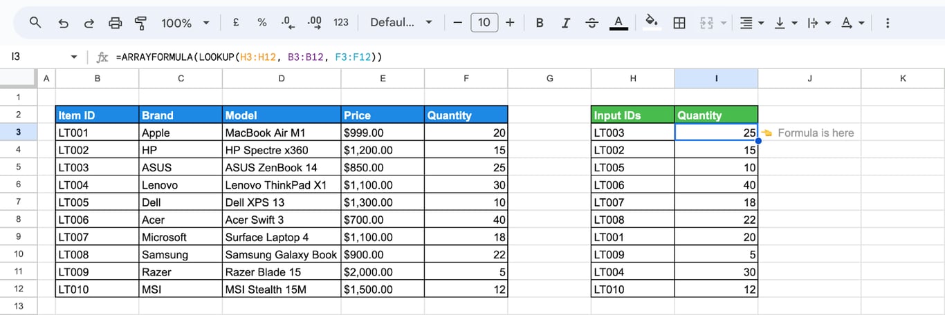
Inside ARRAYFORMULA, LOOKUP takes a range of keys and returns a value for each:
=ARRAYFORMULA(LOOKUP(H3:H12, B3:B12, F3:F12))
- H3:H12: the IDs to look up.
- B3:B12: the item IDs in the table.
- F3:F12: the quantities.
A total for several keys with SUM
Wrap the same formula in SUM to add up the values it returns:
=SUM(ARRAYFORMULA(LOOKUP(H3:H6, B3:B12, F3:F12)))
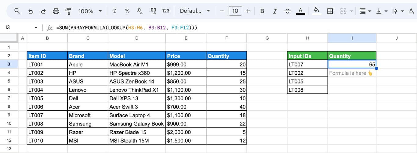
The four IDs have quantities of 18, 15, 10 and 22, and the formula returns 65.
A comparison with IF and AVERAGE
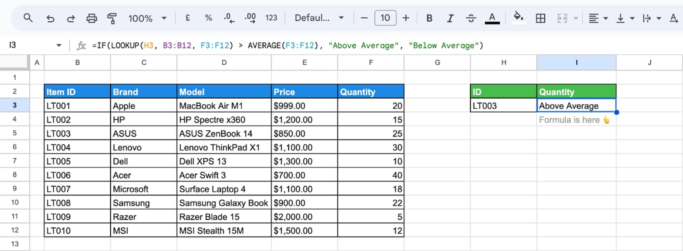
To label an item by whether its quantity is above the average of all items:
=IF(LOOKUP(H3, B3:B12, F3:F12) > AVERAGE(F3:F12), "Above Average", "Below Average")
- LOOKUP(H3, B3:B12, F3:F12): the quantity of the item in H3.
- AVERAGE(F3:F12): the average quantity.
- IF: returns one label or the other; see the guide to the IF function.
The last match in a column
LOOKUP has one well-known use on unsorted data. This formula returns the value of the last row that meets a condition:
=ARRAYFORMULA(LOOKUP(2, 1/(C3:C12 = "Mike"), D3:D12))
The division turns matching rows into 1 and all others into errors. LOOKUP looks for 2, never finds it, and returns the last 1, which is the last matching row. ARRAYFORMULA is required; without it the formula returns a wrong value.
Problems with LOOKUP and how to fix them
Problems with LOOKUP and how to fix them
⚠️ Error: A wrong value, with no error.
✅ Solution: The search range is not sorted in ascending order. Sort the table by the search column, or switch to a lookup with an exact match: =VLOOKUP(H3, B3:D12, 3, FALSE) or =XLOOKUP(H3, B3:B12, D3:D12).
⚠️ Error: A value comes back for a key that is not in the table.
✅ Solution: That is how LOOKUP works: without an exact match it returns the nearest smaller value. If a missing key should be reported as missing, use VLOOKUP with FALSE or XLOOKUP.
⚠️ Error: #N/A
✅ Solution: The key is smaller than every value in the search range, or the range is empty. Check the key and the range.
⚠️ Error: The result comes from the wrong row.
✅ Solution: The search range and the result range do not line up. Both have to start and end in the same rows, B3:B12 with D3:D12, not with D2:D12.
⚠️ Error: Numbers are not found although they are in the list.
✅ Solution: The key is a number and the range holds numbers as text, or the other way round. Convert one side with VALUE or TO_TEXT.
Related Google Sheets functions
Related Google Sheets functions
Functions that are often used instead of LOOKUP, each with its own guide:
- VLOOKUP: Looks down the first column of a table, with an exact-match option.
- HLOOKUP: The same along the first row.
- XLOOKUP vs VLOOKUP: The newer lookup that searches in any direction.
- INDEX and MATCH: A lookup built from two functions.
- MATCH: Returns the position of a value in a range.
- IMPORTRANGE: Brings a range from another spreadsheet into the current one.
- FILTER: Returns every row that meets a condition.
- QUERY vs VLOOKUP: When a query does the job better than a lookup.
A lookup that fails silently is a data problem, not a formula problem
A lookup that fails silently is a data problem, not a formula problem
The wrong model in the unsorted example above is the kind of error nobody notices in a report: the cell is filled, the number looks plausible, and the total is off. Lookups between pasted exports are full of such risks, an order changed by someone, a key spelled differently in two systems, a row added in the middle.
The OWOX Data Marts extension for Google Sheets covers that half. A data analyst publishes a data mart (a table or an SQL query in your data warehouse) and makes it available for reports. In Sheets you open the extension, pick the data mart, tick the columns you want and run it. The rows land in a tab, ready for your formulas.
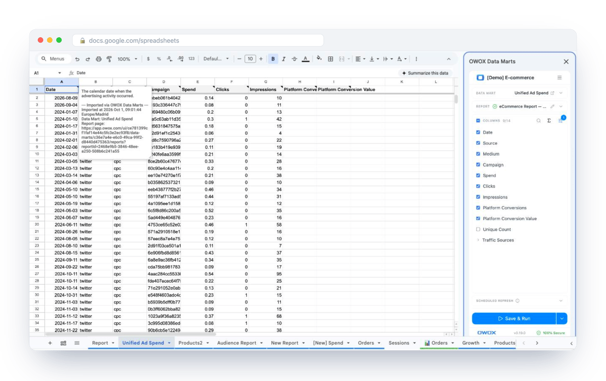
What changes for the person who maintains the sheet:
- Refresh replaces re-export. Refresh current report in the extension menu re-runs the same pull, and a scheduled refresh keeps the tab current without anyone touching it.
- The source is written on the sheet. The header cell of an imported tab carries a note with the data mart it came from, the time of the import and a link to the report.
- No SQL and no warehouse access needed. The analyst decides which data marts and columns are available. You choose from that list.
The extension does not write or change the analyst’s SQL. A join written there once, on a real key, is checked by the people who own the data, and the sheet receives the matched columns on every refresh. The extension comes with the OWOX Cloud plans of OWOX Data Marts; spreadsheet reporting describes both ways data reaches a sheet.
Turn your data into decisions.
Governed data marts give you the clean foundation ML needs to actually work.
- No AI hallucinations
- Analyst-governed definitions
- Every number traces to SQL
Frequently Asked Questions
How does the LOOKUP function handle missing or non-existent data?
LOOKUP searches for the closest match. If an exact match isn’t found, it returns the closest value that's smaller than the search key. If no such value exists, the LOOKUP may return an incorrect result or cause an error, such as #N/A.
What causes the #N/A error in the LOOKUP function, and how can it be resolved?
LOOKUP returns #N/A when the search key is smaller than every value in the search range, or when the range is empty. A key that is simply missing does not give #N/A: LOOKUP returns the nearest smaller value. And unsorted data does not give an error either, it gives a wrong result.
How can you apply the LOOKUP function with sorted data in Google Sheets?
To use LOOKUP effectively, ensure the search range is sorted in ascending order. The function looks for the closest match and retrieves the corresponding value. If the data isn’t sorted, the results may be inaccurate or unexpected.
How does the LOOKUP function compare to VLOOKUP, XLOOKUP, and HLOOKUP?
LOOKUP searches a row or a column but always assumes sorted data and has no exact-match setting. VLOOKUP searches the first column of a table and HLOOKUP the first row; both find exact matches in unsorted data when the last argument is FALSE. XLOOKUP searches in any direction, matches exactly by default and can return a text of your choice when nothing is found.
How do you use the LOOKUP function to find a text string or numeric value in Google Sheets?
Give LOOKUP the key, the range to search and the range to return from: =LOOKUP("Apple", A2:A10, B2:B10) looks for Apple in column A and returns the value from the same row of column B. Column A has to be sorted in ascending order, otherwise the result can be wrong without any error.
What is the LOOKUP function in Google Sheets, and how does it work?
The LOOKUP function in Google Sheets searches for a value in a range and returns a corresponding result from another range. It works by finding the closest match when data is sorted. LOOKUP can search both horizontally and vertically but requires sorted data for accurate results.