VLOOKUP with multiple criteria in Google Sheets: 5 ways

Why VLOOKUP needs help

=VLOOKUP(search_key, range, index, [is_sorted])

• search_key: one value to look for.
• range: the table; the key is searched in its first column.
• index: the number of the column to return.
• is_sorted: FALSE for an exact match.

There is one search key and one column to search, so “John Doe in Human Resources” cannot be asked directly. The basics of the function are in the guide to VLOOKUP.

1. Helper column

Add a column to the table that joins the criteria, and search in it.

=B3 & "|" & C3

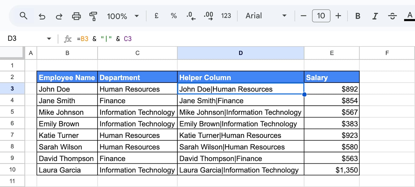
=VLOOKUP(G3 & "|" & H3, $D$3:$E$10, 2, FALSE)

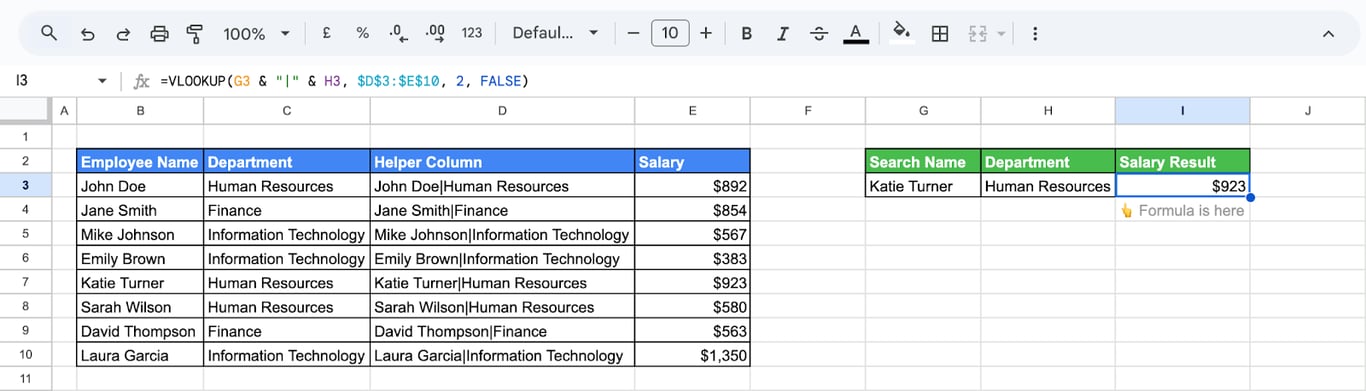
The search key is built the same way as the helper values, with the same separator. The helper column has to be the first column of the lookup range, to the left of the value you want back.

The separator matters. Without it, “Ann” joined with “Abel” and “Anna” joined with “Bel” give the same key, “AnnAbel”. Use a character that cannot occur in the data, such as the vertical bar.

This is the most transparent method: the key is visible in the sheet, and when a lookup fails you can see why.

When the criteria are parts of one column

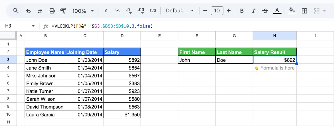
Sometimes the table already holds the combined value, such as a full name, and the criteria arrive in two cells. Then only the search key is joined:

=VLOOKUP(F3 & " " & G3, $B$3:$D$10, 3, FALSE)

2. Array inside VLOOKUP, no helper column

The joined column can be built inside the formula with curly braces: the first column of the array is the joined key, the second the values to return.

=ARRAYFORMULA(VLOOKUP(F3 & "|" & G3, {$B$3:$B$10 & "|" & $C$3:$C$10, $D$3:$D$10}, 2, FALSE))

ARRAYFORMULA is required, because the ranges are joined row by row; without it the formula returns #REF!. The sheet stays free of extra columns, at the price of a formula that is harder to read and to debug.

Do not use CHOOSE for this

A variant copied from Excel builds the same array with CHOOSE:

=ARRAYFORMULA(VLOOKUP(F3 & "|" & G3, CHOOSE({1, 2}, $B$3:$B$10 & "|" & $C$3:$C$10, $D$3:$D$10), 2, FALSE))

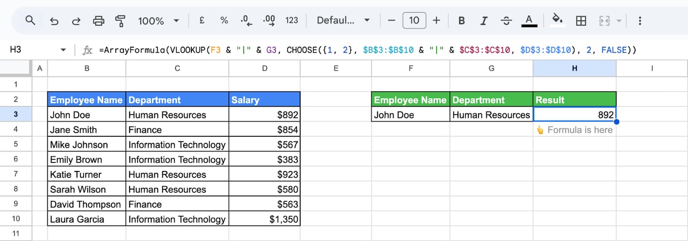
In our test in Google Sheets, CHOOSE with {1, 2} returned only the first row of the two ranges, so the lookup finds a match only when the row you need is the first one, as in the screenshot, and returns #N/A for every other row. Use the curly-brace array above.

Look to the left

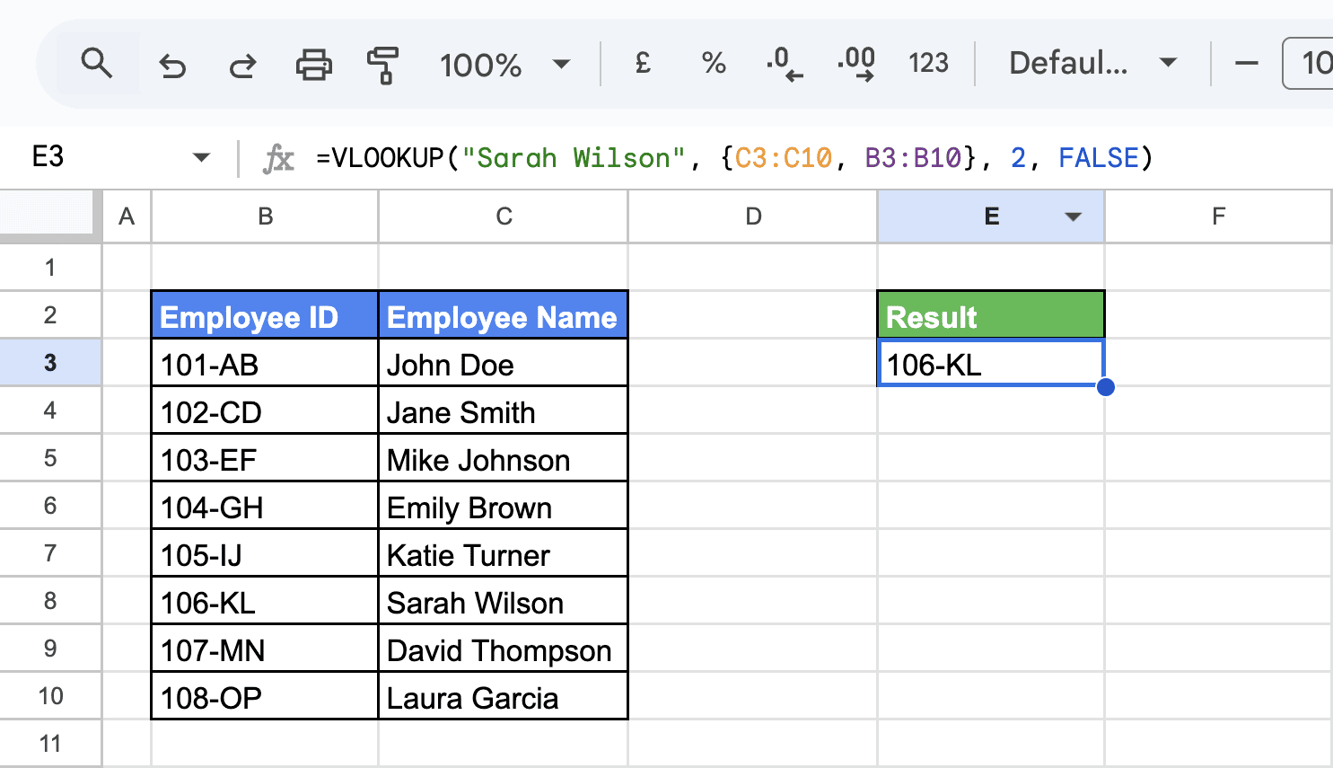
The same curly braces solve another limit of VLOOKUP, that it can only return columns to the right of the key. Put the columns into the array in the order you need:

=VLOOKUP("Sarah Wilson", {C3:C10, B3:B10}, 2, FALSE)

3. FILTER

FILTER takes any number of conditions, and a row must meet all of them:

=FILTER(D3:D10, B3:B10 = F3, C3:C10 = G3)

There is nothing to join and no separator to choose. If several rows match, FILTER returns all of them, one under another, where VLOOKUP would silently return the first. To take only the first match, wrap it in INDEX: =INDEX(FILTER(D3:D10, B3:B10 = F3, C3:C10 = G3), 1).

Conditions are not limited to “equals”: C3:C10 = G3, D3:D10 > 500 works as well. When no row matches, FILTER returns #N/A; wrap it in IFNA to show a text.

4. XLOOKUP

XLOOKUP takes the search range and the result range separately, so the joined key does not need an array with two columns:

=ARRAYFORMULA(XLOOKUP(F3 & "|" & G3, B3:B10 & "|" & C3:C10, D3:D10))

ARRAYFORMULA is needed here too; without it the formula returned #N/A in our test. The fourth argument of XLOOKUP sets what to show when nothing is found: add , "not found" after the result range. See XLOOKUP and VLOOKUP compared.

5. INDEX and MATCH

=INDEX(D3:D10, MATCH(1, (B3:B10 = F3) * (C3:C10 = G3), 0))

Each comparison returns TRUE or FALSE for every row. Multiplied, they give 1 only in the rows where both are true, and MATCH finds the position of the first 1. INDEX returns the salary from that position. More conditions are more brackets multiplied together.

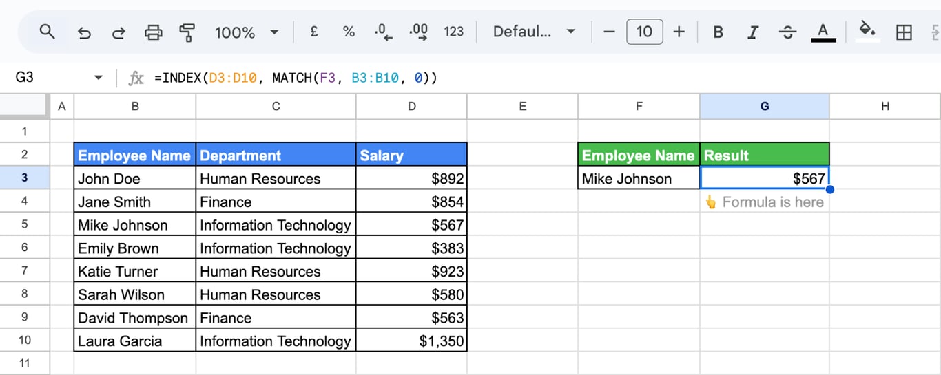
With one criterion, the same pair is the classic alternative to VLOOKUP:

=INDEX(D3:D10, MATCH(F3, B3:B10, 0))

See the guide to MATCH.

When the result is a number: SUMIFS

If the value to return is a number and each combination of criteria occurs once, SUMIFS is the simplest lookup of all:

=SUMIFS(D3:D10, B3:B10, F3, C3:C10, G3)

It returns 0 when nothing matches and the sum when several rows match, so use it only where duplicates are impossible or a total is what you want.

Criteria from dropdowns and partial keys

Dropdown lists

A lookup is easier to use when the criteria cells are dropdowns: the reader picks a value that exists, and typos cannot break the match. Select the cell, click Data > Data validation and add a dropdown from the range that holds the keys.

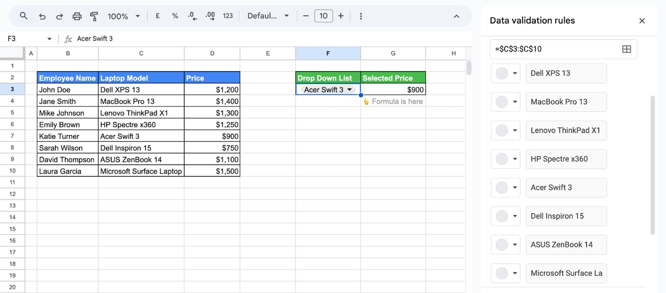
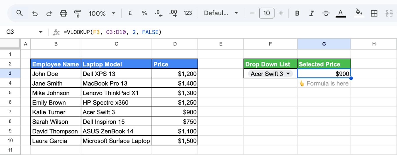
=VLOOKUP(F3, C3:D10, 2, FALSE)

See data validation.

A key that is only the beginning of the value

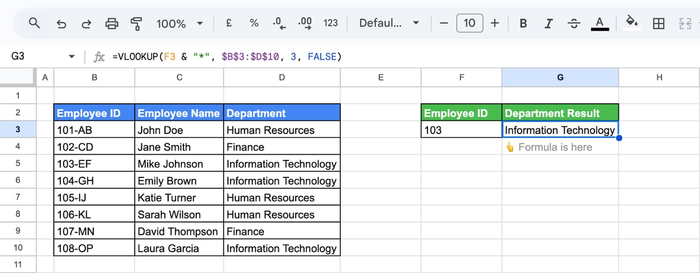
With an exact match, VLOOKUP accepts wildcards in the search key. An asterisk after the key finds the first value that starts with it:

=VLOOKUP(F3 & "*", $B$3:$D$10, 3, FALSE)

Errors and wrong results

⚠️ Error: #N/A

✅ Solution: No row has this combination. Check the separator (the key and the helper column must use the same one), spaces at the ends of the values, and numbers stored as text on one side. Dates join as serial numbers, which is fine as long as both sides are real dates.

⚠️ Error: #REF! in the array version.

✅ Solution: ARRAYFORMULA is missing around a formula that joins two ranges inside curly braces.

⚠️ Error: #REF! although ARRAYFORMULA is in place.

✅ Solution: The index is larger than the number of columns in the range. With a two-column array, the index is 2. An index of 0 returns #VALUE!.

⚠️ Error: The formula returns a value, but from the wrong row.

✅ Solution: Two causes. The last argument is TRUE or missing, which makes VLOOKUP return an approximate match: set it to FALSE. Or the combination occurs more than once and the first match is returned: use FILTER to see all of them.

⚠️ Error: The lookup worked for the first row and fails for the others.

✅ Solution: The ranges are not locked. Add dollar signs, $B$3:$D$10, before copying the formula down.

Related guides

• VLOOKUP: The function itself, with exact and approximate match.
• VLOOKUP with IF: Conditions around a lookup.
• XLOOKUP and VLOOKUP: What the newer function adds.
• QUERY and VLOOKUP: When a query is the better lookup.
• FILTER: Rows that meet several conditions.
• MATCH: The position of a value in a range.
• Array formulas: Curly braces and ARRAYFORMULA.
• HLOOKUP: The same lookup across a row.

A lookup by two keys is a join done by hand

Matching a salary to a name and a department, or a cost to a campaign and a date, is a join between two tables. In a sheet it is rebuilt with every export: paste both tables, rebuild the keys, fix the rows that do not match because of a space. In a data warehouse the same join is one line of SQL that runs the same way every time.

The OWOX Data Marts extension for Google Sheets covers that half. A data analyst publishes a data mart (a table or an SQL query in your data warehouse) and makes it available for reports. In Sheets you open the extension, pick the data mart, tick the columns you want and run it. The rows land in a tab, ready for your formulas.

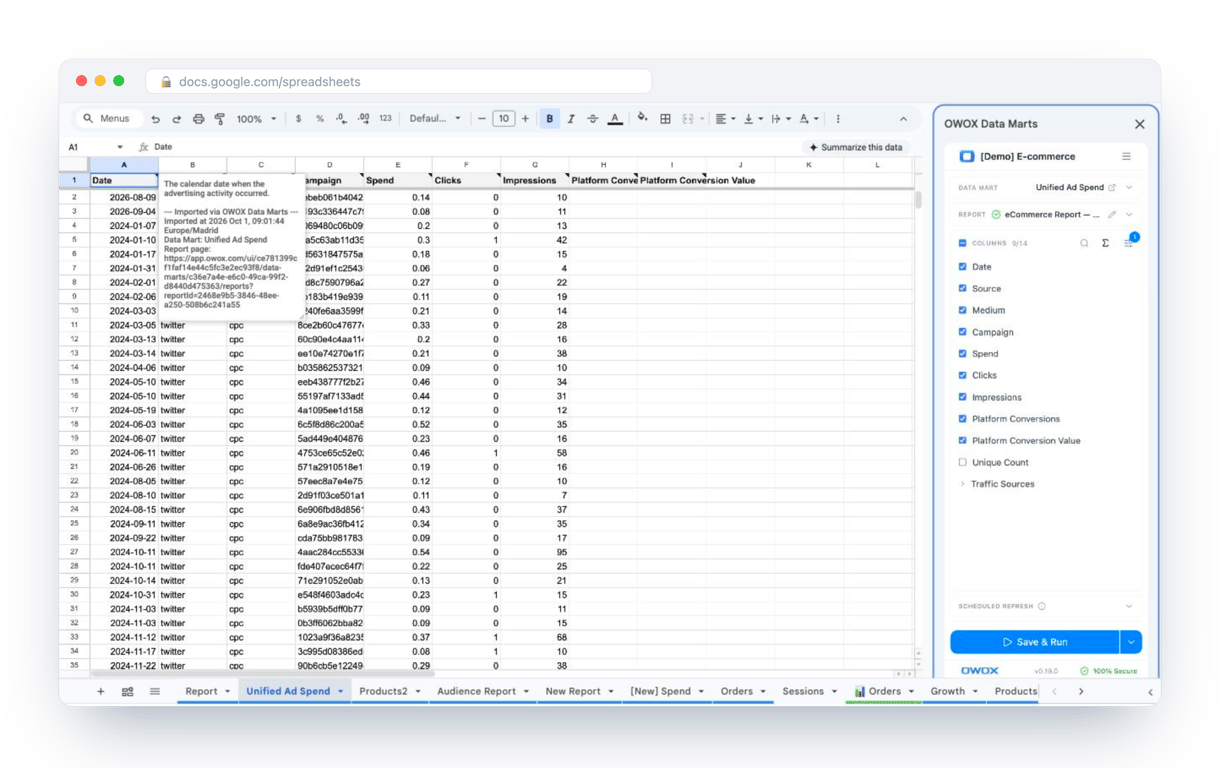
What changes for the person who maintains the sheet:

• Refresh replaces re-export. Refresh current report in the extension menu re-runs the same pull, and a scheduled refresh keeps the tab current without anyone touching it.
• The source is written on the sheet. The header cell of an imported tab carries a note with the data mart it came from, the time of the import and a link to the report.
• No SQL and no warehouse access needed. The analyst decides which data marts and columns are available. You choose from that list.

The extension does not write or change the analyst’s SQL. With the join written once in that SQL, the sheet receives one table that already has both sets of columns, and the two-key lookup is no longer needed. The extension comes with the OWOX Cloud plans of OWOX Data Marts; spreadsheet reporting describes both ways data reaches a sheet.

Google Sheets TipsLOOKUP function in Google Sheets: syntax, examples, limitsOctober 2, 2026→Google Sheets TipsINDEX MATCH in Google Sheets: formula, examples and errorsOctober 2, 2026→Google Sheets TipsIF with VLOOKUP in Google Sheets: formulas and examplesOctober 2, 2026→

See all articles →