IFS function in Google Sheets: several conditions in one formula
IFS checks several conditions in order and returns the value that belongs to the first one that is true. It replaces a chain of nested IF functions. This guide shows the syntax, why the order of the conditions matters, how to add a default with TRUE, how to combine conditions with AND and OR, and why IFS returns #N/A.

IFS checks several conditions one after another and returns the value that belongs to the first condition that is true:
=IFS(C3 >= 90, "A", C3 >= 80, "B", C3 >= 70, "C", C3 >= 60, "D", TRUE, "F")
A score of 85 fails the first test, passes the second and gets “B”. The last pair, TRUE, "F", is the default: it catches everything the earlier conditions did not.
IFS does the job of nested IF functions without the nesting. The same grading written with IF needs four functions and four closing brackets: =IF(C3>=90,"A",IF(C3>=80,"B",IF(C3>=70,"C",IF(C3>=60,"D","F")))).
IFS syntax
=IFS(condition1, value1, [condition2, value2, ...])
- condition1: a test that is TRUE or FALSE, such as
C3 >= 90. - value1: what to return when condition1 is true.
- condition2, value2, …: more pairs, checked in the order they are written.
Three rules follow from “the first true condition wins”:
- Order matters. Put the strictest condition first.
=IFS(C3 > 1000, "Medium", C3 > 2000, "High")never returns “High”, because every number above 2000 is also above 1000 and stops at the first pair. - There is no “otherwise” argument. If no condition is true, IFS returns #N/A. Add
TRUE, "value"as the last pair to set a default. - Later pairs are not evaluated. Once a condition is true, the rest of the formula is skipped, so an error further down the list does no harm.
Examples
Grades from scores
=IFS(C3>=90, "A", C3>=80, "B", C3>=70, "C", C3>=60, "D", C3<59, "F")
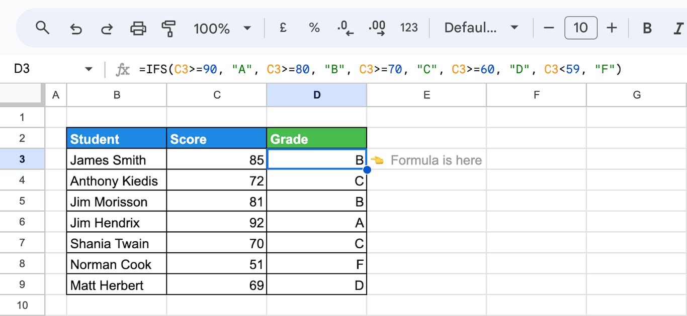
The formula in the screenshot works for the scores in the table and has a gap: the last condition is C3<59, so a score of exactly 59, or 59.5, matches nothing and returns #N/A. Close the scale with a default instead of a last condition:
=IFS(C3>=90, "A", C3>=80, "B", C3>=70, "C", C3>=60, "D", TRUE, "F")
Categories from thresholds
=IFS(C3 > 10000, "High", C3 >= 5000, "Medium", TRUE, "Low")
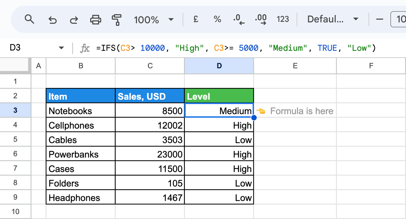
For a long list of thresholds, a lookup table with an approximate match is easier to maintain than a long IFS: the thresholds sit in cells where anyone can change them. See VLOOKUP and LOOKUP.
Several tests in one condition: AND and OR
A condition can combine tests. AND is true when all of them are, OR when at least one is:
=IFS(AND(C3 >= 4, D3 >= 3), "High", AND(C3 >= 3, D3 >= 2), "Medium", TRUE, "Low")
With urgency in column C and impact in column D, a task is “High” when both scores are high, “Medium” when both are at least moderate, and “Low” otherwise. Check that every reference points to the row of the formula: a condition that reads C2 in a formula on row 3 rates each task by the scores of the task above it, and nothing warns about it.
A condition on a looked-up value
=IFS(VLOOKUP(F3, B3:D7, 3, FALSE)="Sales", "Sales Employee", VLOOKUP(F3, B3:D7, 3, FALSE)="Marketing", "Marketing Employee")
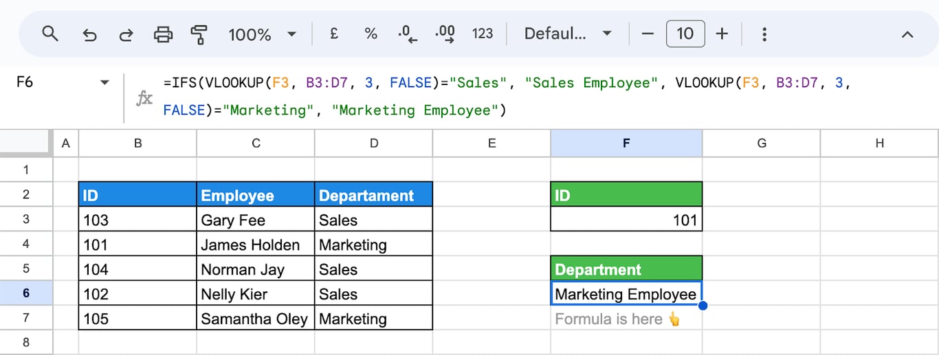
The lookup is repeated in every condition. LET names the result once and makes the formula shorter and faster to read:
=LET(dept, VLOOKUP(F3, B3:D7, 3, FALSE), IFS(dept="Sales", "Sales Employee", dept="Marketing", "Marketing Employee", TRUE, "Other"))
A whole column
=ARRAYFORMULA(IFS(C3:C12 >= 5000, "High", C3:C12 >= 1000, "Medium", TRUE, "Low"))
Inside ARRAYFORMULA, IFS evaluates the conditions row by row and fills the column from one formula.
OWOX Data Marts
See your first report built in real time. 15 minutes.
- Connect your data warehouse
- Pick your metrics
- Get a live Google Sheets report
In the time it takes to write a ticket. Then imagine never writing that ticket again.
Book a DemoWe'll use your actual use case
IFS, nested IF or SWITCH
| Situation | Use |
|---|---|
| One condition, two outcomes | IF |
| Several conditions with ranges (greater than, less than) | IFS |
| One cell compared with a list of exact values | SWITCH |
| Many thresholds that change over time | A lookup table with VLOOKUP or LOOKUP |
SWITCH compares one expression with a list of values and has a real default argument at the end:
=SWITCH(B3, "N", "North", "S", "South", "E", "East", "W", "West", "Unknown")
The same in IFS would repeat B3 = in every pair.
Errors in IFS
⚠️ Error: #N/A
✅ Solution: Either no condition was true, or the arguments are not in pairs. Add a final TRUE, "default", and check that every condition has its value. To keep the formula as it is and replace the error, wrap it: =IFNA(IFS(...), "Other").
⚠️ Error: The same result in every row, or a “wrong” category.
✅ Solution: A broad condition comes before a narrow one. Reorder the pairs from the strictest to the loosest.
⚠️ Error: An empty cell gets a category.
✅ Solution: An empty cell counts as 0 in a comparison, so it passes tests such as C3 < 60. Test for it first: =IFS(C3="", "", C3>=90, "A", ...).
⚠️ Error: Text passes a “greater than” test.
✅ Solution: In a comparison, any text is greater than any number, so “n/a” > 5000 is true. Check with ISNUMBER first, or clean the column.
⚠️ Error: #DIV/0! or another error from the formula.
✅ Solution: A condition that is reached contains the error. Conditions after the first true one are skipped, but the ones before it are all calculated.
Related Google Sheets functions
Related Google Sheets functions
- IF: One condition, two outcomes.
- VLOOKUP with IF: Conditions around a lookup.
- LOOKUP: Tiers from a sorted table.
- COUNTIF and COUNTIFS: Count the rows that meet conditions.
- SUM functions: SUMIF and SUMIFS.
- Array formulas: One formula for a whole column.
- Data validation: Keep the categories consistent.
Business rules written in cells drift apart
Business rules written in cells drift apart
An IFS formula is a business rule: what counts as a high-value order, which score is a pass. Written into a sheet, the rule is copied with every copy of the file, and sooner or later two reports use two versions of “High”. The rows are the same; the answers differ.
The OWOX Data Marts extension for Google Sheets covers that half. A data analyst publishes a data mart (a table or an SQL query in your data warehouse) and makes it available for reports. In Sheets you open the extension, pick the data mart, tick the columns you want and run it. The rows land in a tab, ready for your formulas.
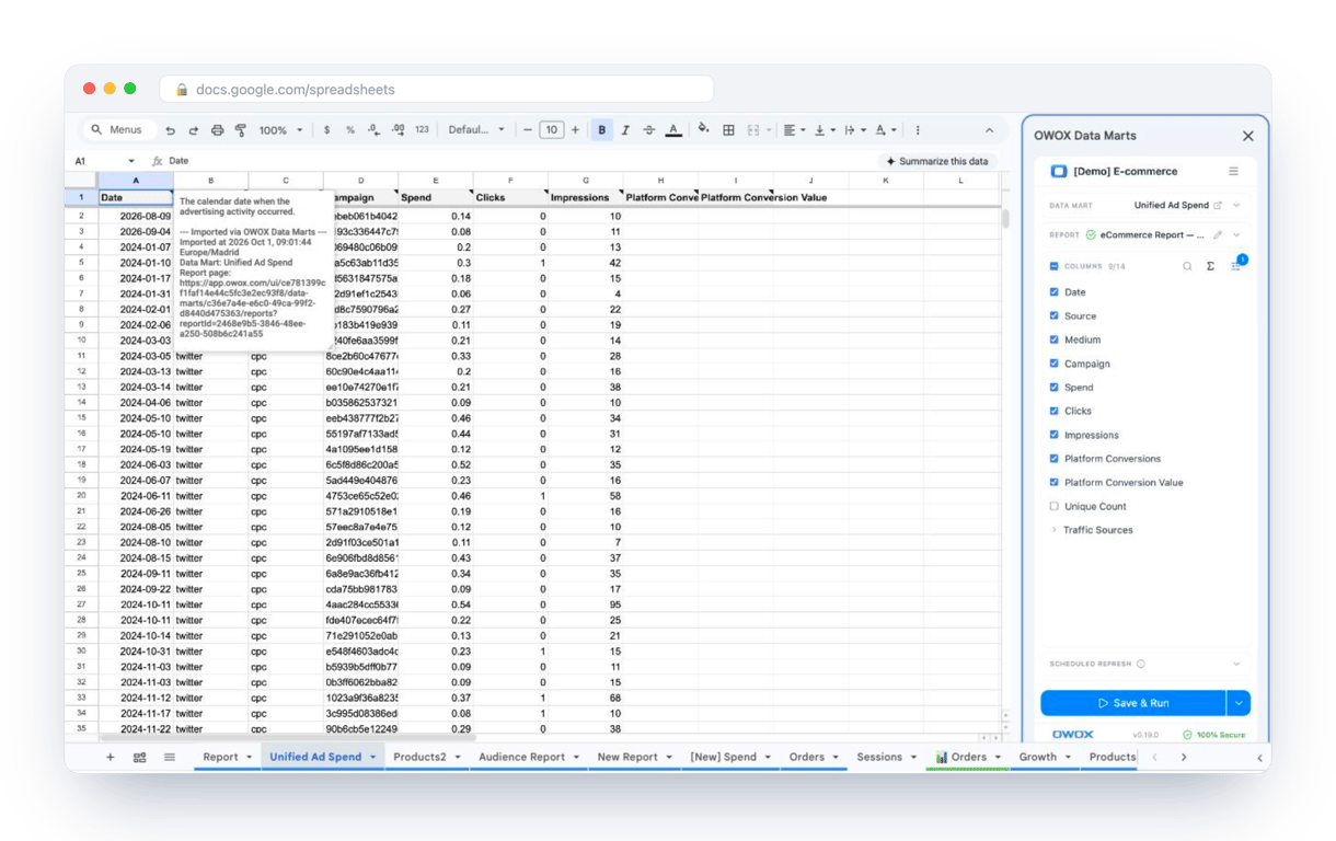
What changes for the person who maintains the sheet:
- Refresh replaces re-export. Refresh current report in the extension menu re-runs the same pull, and a scheduled refresh keeps the tab current without anyone touching it.
- The source is written on the sheet. The header cell of an imported tab carries a note with the data mart it came from, the time of the import and a link to the report.
- No SQL and no warehouse access needed. The analyst decides which data marts and columns are available. You choose from that list.
The extension does not write or change the analyst’s SQL. When the category is calculated once in that SQL, every sheet receives the same label in a column, and IFS is left for the local, one-off classification. The extension comes with the OWOX Cloud plans of OWOX Data Marts; spreadsheet reporting describes both ways data reaches a sheet.
Turn your data into decisions.
Governed data marts give you the clean foundation ML needs to actually work.
- No AI hallucinations
- Analyst-governed definitions
- Every number traces to SQL
Frequently Asked Questions
Are there limitations to the number of conditions the IFS function can handle in Google Sheets?
Yes, the IFS function in Google Sheets can handle up to 127 pairs of conditions and corresponding values. This limit ensures efficient use for most scenarios but requires careful planning when dealing with extensive sets of conditions to avoid exceeding the maximum allowed pairs.
How to use the IFS function in Google Sheets?
To use the IFS function in Google Sheets, structure it as follows: =IFS(condition1, value_if_true1, condition2, value_if_true2, ..., conditionN, value_if_trueN).Specify multiple conditions and their corresponding values to return if true. Include a final condition or value to handle cases where none of the specified conditions are met.
What are the differences between the IFS function and the traditional IF function?
The IFS function in Google Sheets allows for evaluating multiple conditions in a single formula without nesting. In contrast, the traditional IF function is limited to handling one condition per formula, requiring nested IF statements for multiple conditions, which can make formulas more complex and harder to manage.
What exactly does the IFS function do in Google Sheets?
The IFS function evaluates multiple conditions and returns a value corresponding to the first true condition. It simplifies complex logical tests by eliminating the need for nested IF statements, making it easier to manage and understand conditional logic in spreadsheets.
Can the IFS function be used to handle multiple conditions in one column?
Yes, the IFS function in Google Sheets is ideal for handling multiple conditions within a single column. It evaluates each condition sequentially and returns the corresponding value for the first true condition, simplifying complex logic without needing nested IF statements.
How do I write a basic IFS function formula in Google Sheets?
List the conditions and their values in pairs, in the order they should be checked: =IFS(C3>=90, "A", C3>=80, "B", C3>=70, "C", TRUE, "F"). The first condition that is true decides the result, so put the strictest one first. End with TRUE and a default value: without it, a row that meets no condition returns #N/A.