Date functions in Google Sheets: DATE, DATEVALUE, DATEDIF, EDATE and EPOCHTODATE
DATE builds a date from a year, a month and a day. DATEVALUE converts a text into a date. DATEDIF counts the years, months or days between two dates. EDATE moves a date by a number of months, and EPOCHTODATE converts a Unix timestamp. This guide shows the syntax and tested behaviour of each, with the units of DATEDIF and the errors to expect.
Five functions cover most date work in Google Sheets:
| Function | What it does | Example | Result |
|---|---|---|---|
DATE(year, month, day) |
Builds a date from three numbers | =DATE(2024, 3, 1) |
1 March 2024 |
DATEVALUE(date_text) |
Converts a text into a date | =DATEVALUE("2024-09-15") |
15 September 2024 |
DATEDIF(start, end, unit) |
Counts years, months or days between two dates | =DATEDIF(DATE(2020,1,15), DATE(2024,3,1), "Y") |
4 |
EDATE(start, months) |
Moves a date by a number of months | =EDATE(DATE(2024,1,31), 1) |
29 February 2024 |
EPOCHTODATE(timestamp, [unit]) |
Converts a Unix timestamp into a date and time | =EPOCHTODATE(1579046400) |
15 January 2020, 00:00 |
A date in Sheets is a number: the count of days since 30 December 1899. That is why dates can be subtracted and compared, and why a date function sometimes shows a number such as 45000 until the cell is given a date format (Format > Number > Date). The guide to dates and times explains the storage in detail.
DATE: build a date
=DATE(year, month, day)
=DATE(D3, E3, F3)
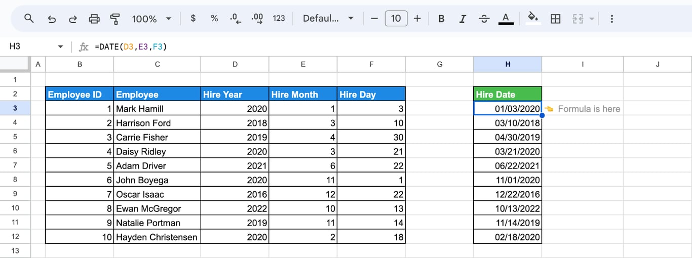
DATE is the safe way to write a date inside a formula, because it does not depend on the locale of the spreadsheet the way a typed “3/1/2024” does. Three behaviours are worth knowing:
- Overflow is carried over.
=DATE(2024, 14, 1)returns 1 February 2025, and=DATE(2024, 2, 30)returns 1 March 2024. This makes arithmetic easy:=DATE(YEAR(A2), MONTH(A2) + 1, 1)is the first day of the next month, also in December. - Use four digits for the year.
=DATE(24, 1, 1)returns a date in 1924. - The result is a real date. It can be subtracted from another date or compared with TODAY.
Days until a date
=DATE(D3, E3, F3) - TODAY()
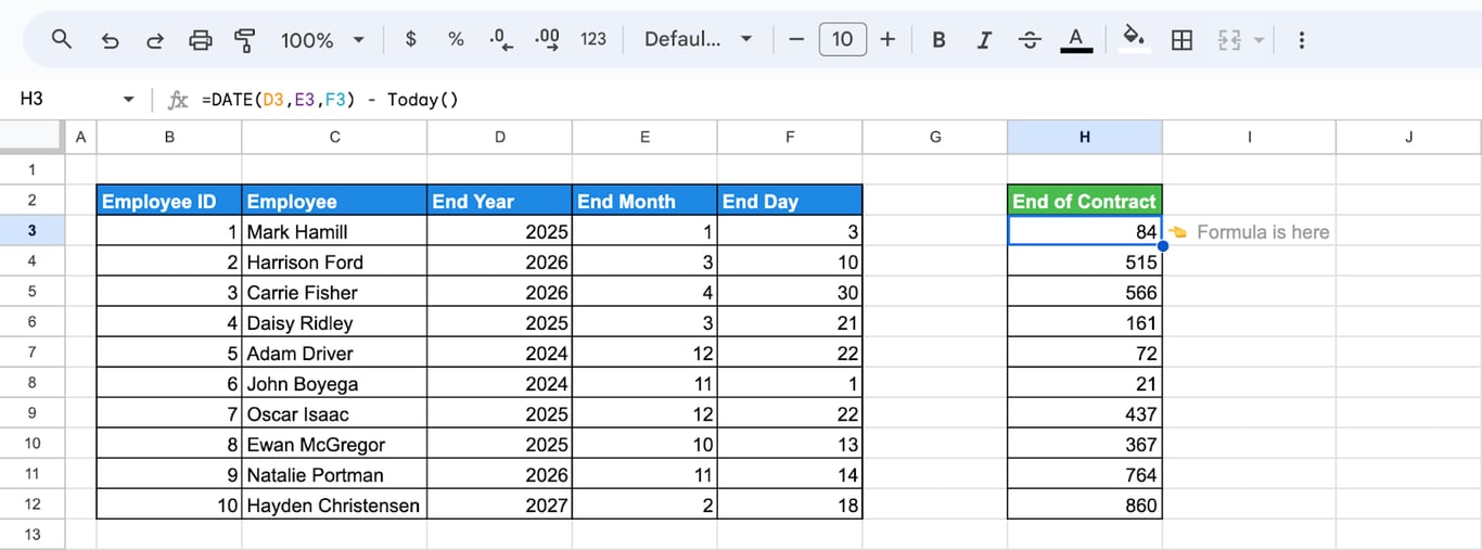
Subtracting two dates gives the days between them. TODAY changes every day, so the result counts down by itself.
Weekday or weekend
=IF(OR(WEEKDAY(DATE(D3, E3, F3))=1, WEEKDAY(DATE(D3, E3, F3))=7), "Weekend", "Weekday")
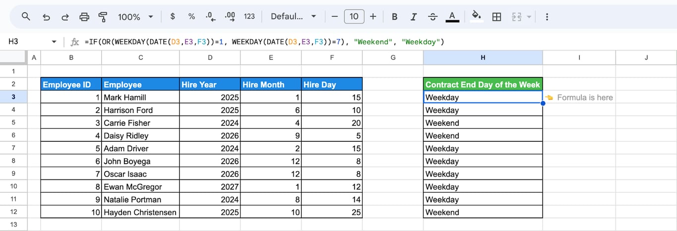
WEEKDAY returns 1 for Sunday and 7 for Saturday. A shorter form of the same test is =IF(WEEKDAY(A2, 2) > 5, "Weekend", "Weekday"), where the second argument makes Monday day 1.
DATEVALUE: convert text into a date
DATEVALUE: convert text into a date
=DATEVALUE(date_text)
Dates that arrive as text (left-aligned, not sortable as dates) are converted with DATEVALUE.
=DATEVALUE(D3)
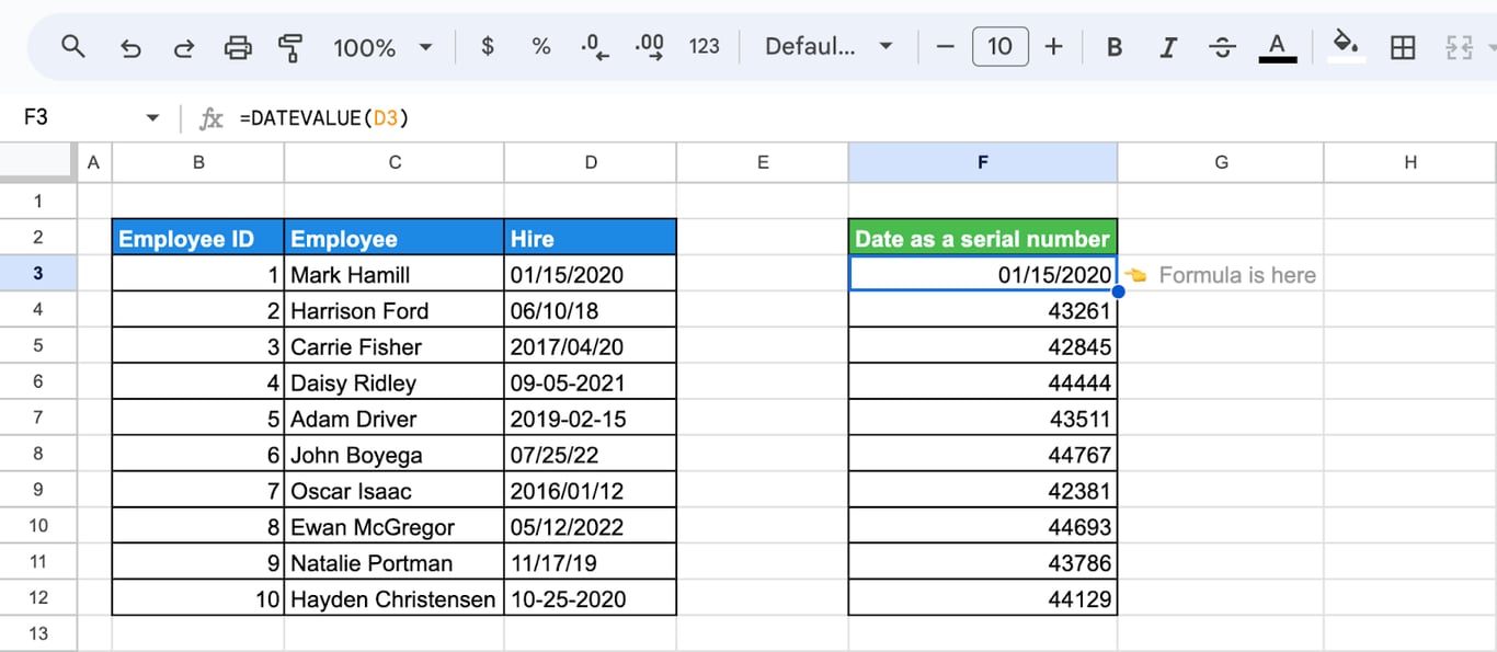
The first result has a date format; the others show the underlying serial numbers. They are correct dates, waiting for a format.
DATEVALUE reads the layouts that Sheets itself understands in the locale of the spreadsheet: “2024-09-15”, “15 August 2024”, “12/10/2023”. A text without a year gets the current year:
=DATEVALUE(E3)
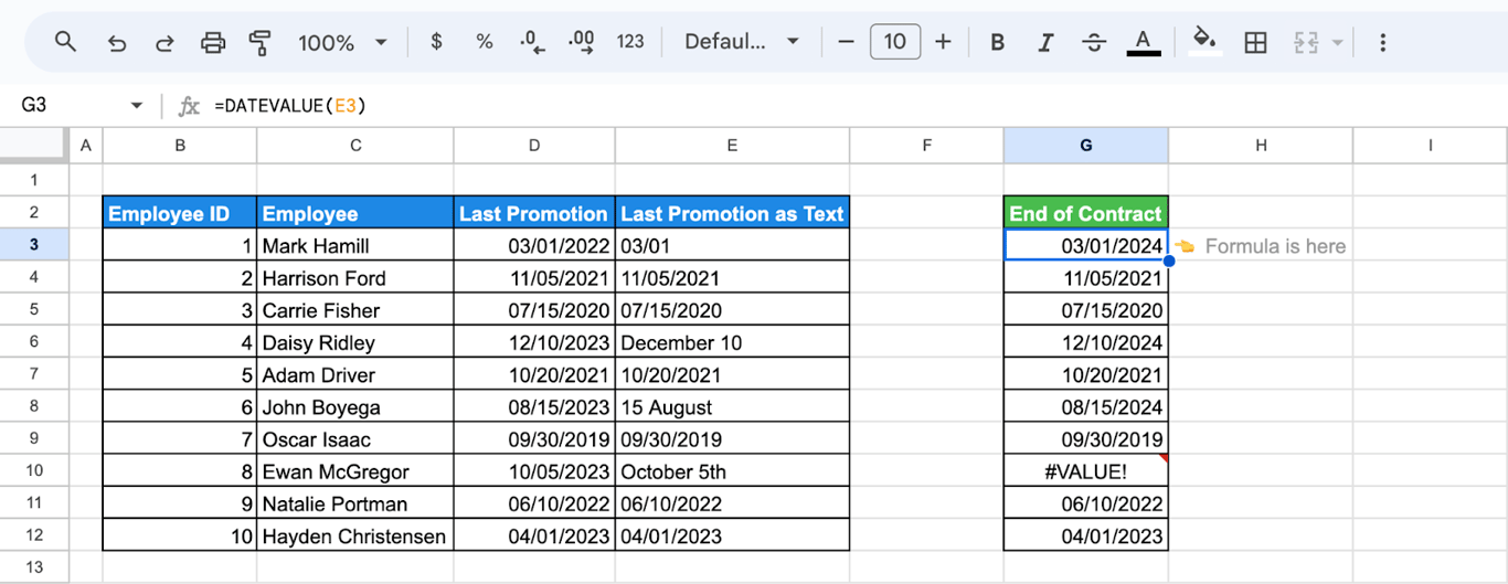
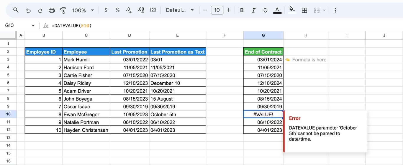
A text it cannot read returns #VALUE!. “October 5th” fails because of the “th”:
Two limits:
- An ambiguous text such as “03/04/2024” is read by the locale: 4 March in the United States, 3 April in most of Europe. If the source used the other order, DATEVALUE returns a valid but wrong date, without an error. Rebuild such dates from their parts with DATE and LEFT, RIGHT and MID.
- DATEVALUE drops the time. For a text with a time, add TIMEVALUE:
=DATEVALUE(A2) + TIMEVALUE(A2).
A date inside a longer text
=DATEVALUE(MID(D3, 11, 10))
For “Hired on: 2019-12-29”, MID takes ten characters starting from the eleventh, “2019-12-29”, and DATEVALUE converts them. Count the start position carefully: one character too early and the last digit of the day is cut off, which still gives a valid date, the wrong one.
OWOX Data Marts
See your first report built in real time. 15 minutes.
- Connect your data warehouse
- Pick your metrics
- Get a live Google Sheets report
In the time it takes to write a ticket. Then imagine never writing that ticket again.
Book a DemoWe'll use your actual use case
DATEDIF: years, months and days between two dates
DATEDIF: years, months and days between two dates
=DATEDIF(start_date, end_date, unit)
The unit decides what is counted. For 15 January 2020 to 1 March 2024:
| Unit | Counts | Result |
|---|---|---|
"Y" |
Complete years | 4 |
"M" |
Complete months | 49 |
"D" |
Days | 1507 |
"YM" |
Months left after the complete years | 1 |
"MD" |
Days left after the complete months | 15 |
"YD" |
Days, as if both dates were in the same year | 46 |
The start date has to come first. If it is later than the end date, DATEDIF returns #NUM!.
Days
=DATEDIF(D3, E3, "D")
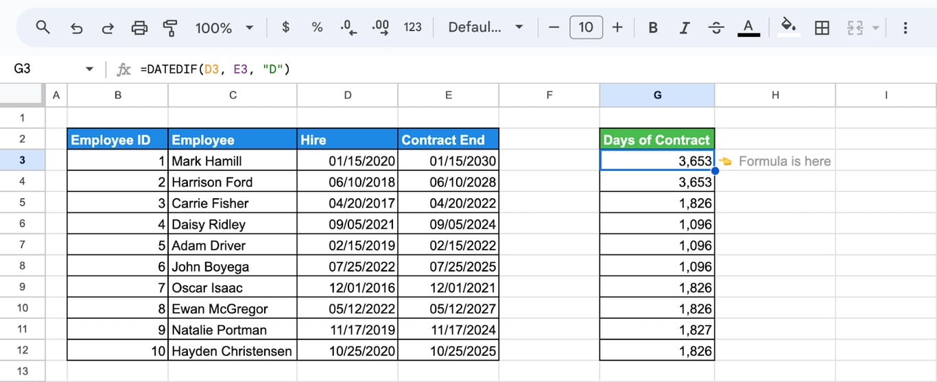
With “D”, DATEDIF gives the same number as subtracting the dates, =E3-D3, or as DAYS. Counted up to today:
=DATEDIF(D3, TODAY(), "D")
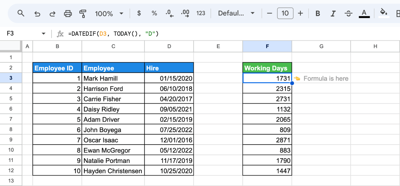
These are calendar days. For working days, use NETWORKDAYS.
Months
=DATEDIF(D3, F3, "M")
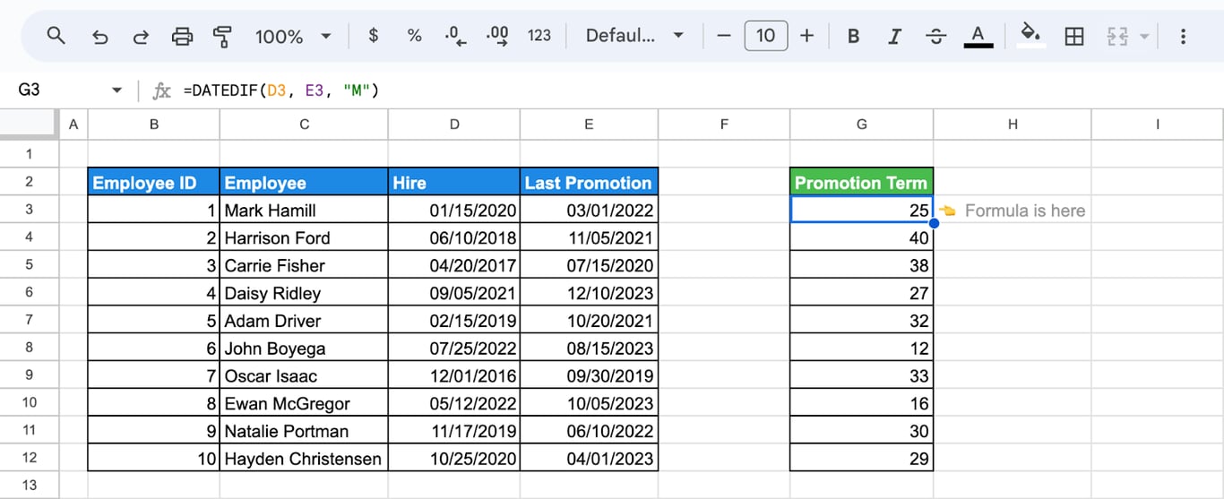
Only complete months count: from 15 January to 14 March is one month, from 15 January to 15 March two.
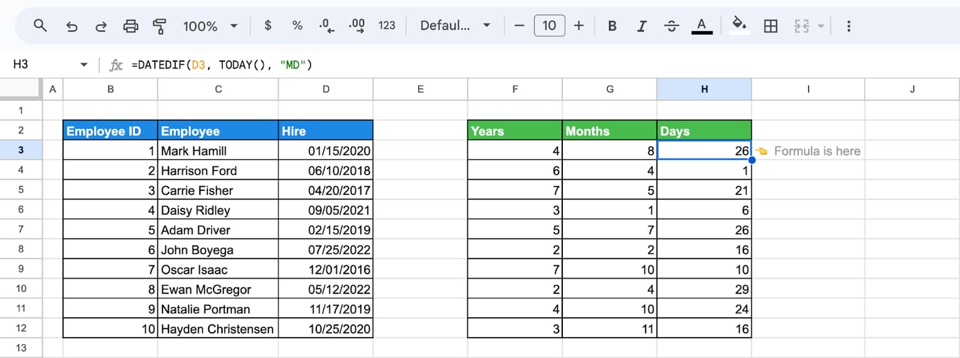
Tenure or age in years, months and days
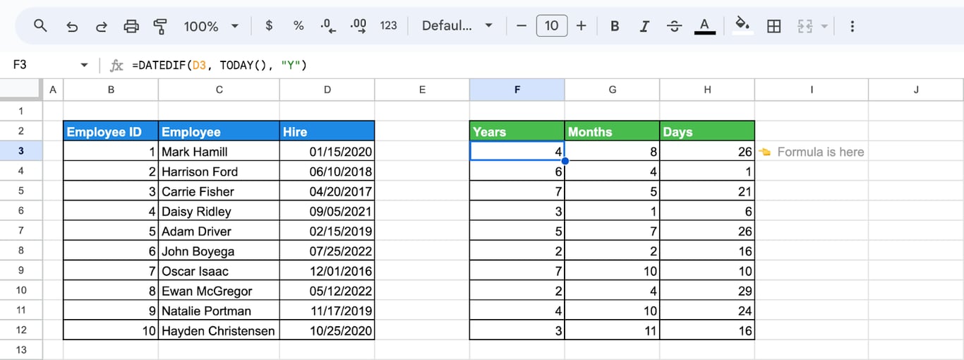
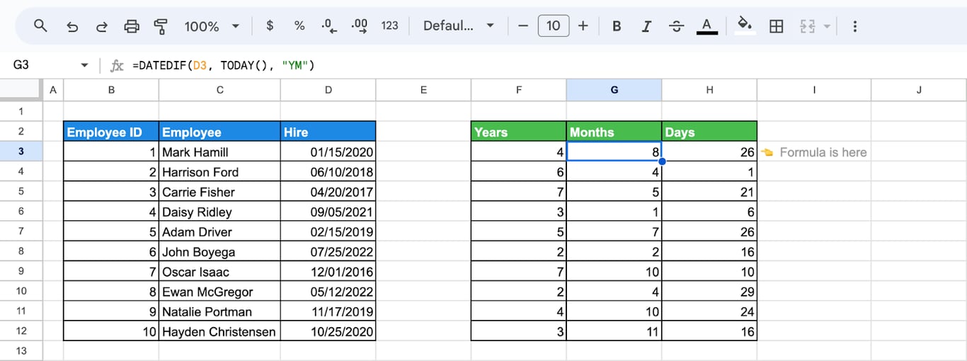
Three formulas with three units give the full breakdown:
=DATEDIF(D3, TODAY(), "Y")
=DATEDIF(D3, TODAY(), "YM")
=DATEDIF(D3, TODAY(), "MD")
Joined into one text:
=DATEDIF(D3, TODAY(), "Y") & " years, " & DATEDIF(D3, TODAY(), "YM") & " months, " & DATEDIF(D3, TODAY(), "MD") & " days"
The same formula with a birth date returns an age. =DATEDIF(A2, TODAY(), "Y") alone is the age in whole years.
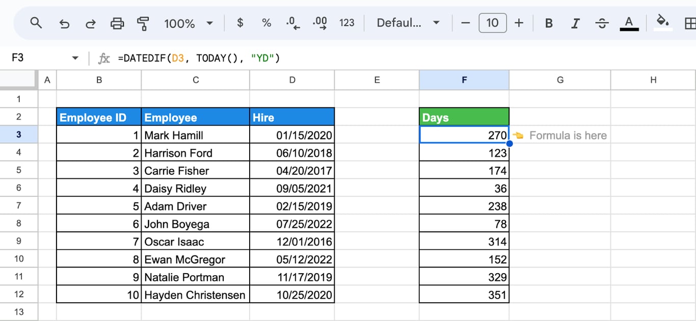
Days since the last anniversary
=DATEDIF(D3, TODAY(), "YD")
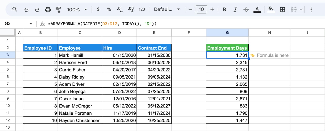
A whole column
=ARRAYFORMULA(DATEDIF(D3:D12, TODAY(), "D"))
EDATE: add or subtract months
=EDATE(start_date, months)
=EDATE(E3, 6)
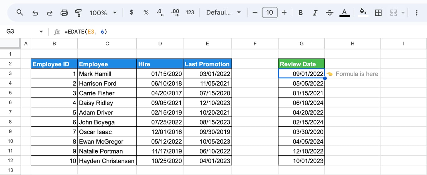
A negative number goes back: =EDATE(E3, -3). EDATE keeps the day of the month, and when the target month is shorter, it returns its last day: one month after 31 January 2024 is 29 February 2024. For years, multiply: =EDATE(A2, 12) is the same day next year.
EDATE is the right tool for renewal dates, trial ends and review dates, where “plus 30 days” would drift.
The length of a period that starts on a date
=EDATE(D3, 1) - D3
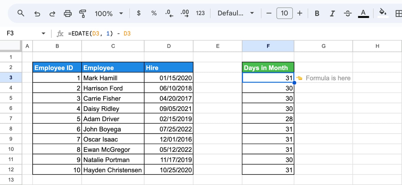
The result is the number of days from the date to the same day next month. For the last day of a month, use EOMONTH.
EPOCHTODATE: convert a unix timestamp
EPOCHTODATE: convert a unix timestamp
=EPOCHTODATE(timestamp, [unit])
- timestamp: a Unix timestamp, the time elapsed since 1 January 1970, 00:00 UTC.
- unit: optional. 1, the default, for seconds; 2 for milliseconds; 3 for microseconds.
=EPOCHTODATE(E3)
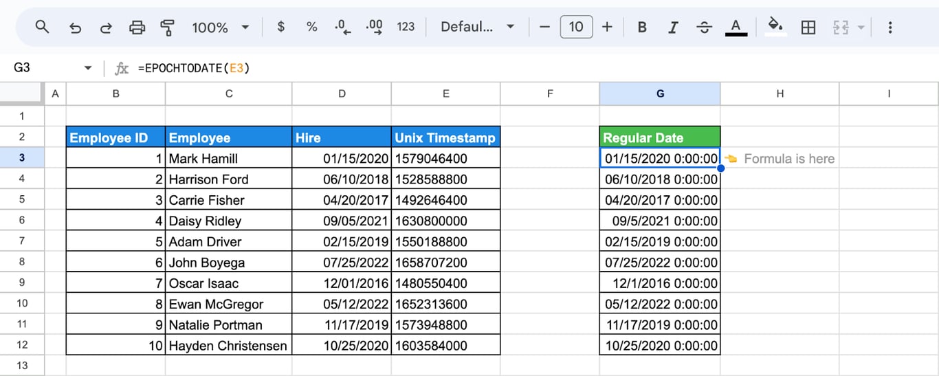
Timestamps from APIs and logs are often in milliseconds, three digits longer. Set the unit to 2:
=EPOCHTODATE(E3, 2)
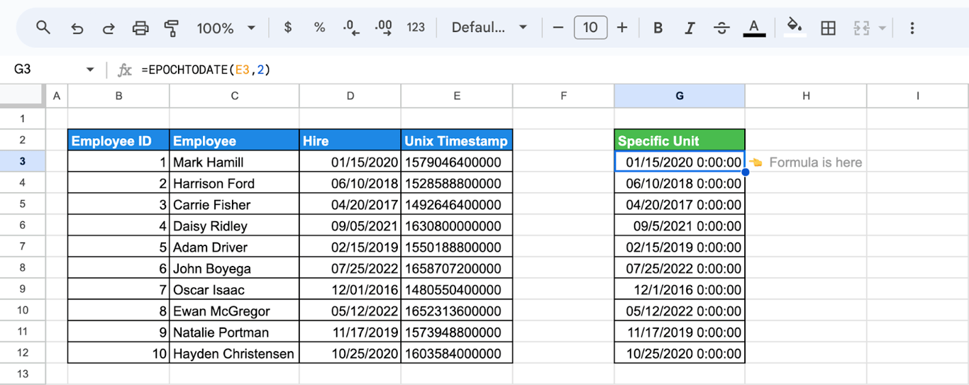
The result is in UTC, not in the time zone of the spreadsheet. To shift it, add the offset as a fraction of a day: =EPOCHTODATE(E3) + 2/24 for UTC+2.
The reverse, from a date to a timestamp in seconds:
=(D3 - DATE(1970,1,1)) * 86400
Show a date in another format
A date function returns a number with a date format. To write the date in a specific layout inside a text or a label, use TEXT:
=TEXT(E3, "DD MMMM, YYYY")
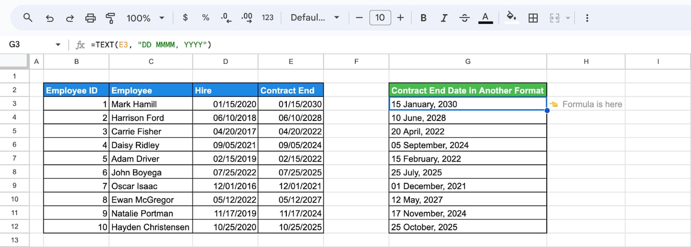
The result of TEXT is a text: good for display, not for further date arithmetic.
Errors with date functions
⚠️ Error: #VALUE!
✅ Solution: A text could not be read as a date: an ordinal such as “5th”, a month name in another language than the spreadsheet’s locale, or a stray character. Clean the text or rebuild the date with DATE.
⚠️ Error: #NUM! in DATEDIF.
✅ Solution: The start date is later than the end date, or the unit is not one of “Y”, “M”, “D”, “YM”, “MD”, “YD”.
⚠️ Error: A number such as 45000 appears where a date should be.
✅ Solution: The value is a date without a date format. Apply Format > Number > Date.
⚠️ Error: The date is valid, but the day and the month are swapped.
✅ Solution: A text date was read in the wrong order for its source. Check File > Settings > Locale, or build the date from its parts.
⚠️ Error: A date lands in the 1900s.
✅ Solution: The year was given with two digits. Use four.
⚠️ Error: A timestamp converts to a date in 1970 or far in the future.
✅ Solution: The unit does not match: seconds were read as milliseconds or the other way round. Count the digits; a current timestamp has 10 digits in seconds and 13 in milliseconds.
Related Google Sheets functions
Related Google Sheets functions
- Dates and times: How Sheets stores and formats them.
- NOW and TODAY: The current date and time.
- DAY, DAYS and DAYS360: The day of the month and days between dates.
- MONTH and EOMONTH: The month of a date and the last day of a month.
- YEAR and YEARFRAC: The year and the fraction of a year.
- WORKDAY and NETWORKDAYS: Working days.
- Date filtering with QUERY: Rows from a date range.
- TEXT: Format codes for dates.
Dates break at the border between systems
Dates break at the border between systems
Most date problems in a sheet are import problems: an export writes dates as text, in the order of another locale, or as Unix timestamps, and DATEVALUE and EPOCHTODATE are used to repair them. The repair has to be repeated with every export, and one file read in the wrong locale puts April where March should be without any error.
The OWOX Data Marts extension for Google Sheets covers that half. A data analyst publishes a data mart (a table or an SQL query in your data warehouse) and makes it available for reports. In Sheets you open the extension, pick the data mart, tick the columns you want and run it. The rows land in a tab, ready for your formulas.
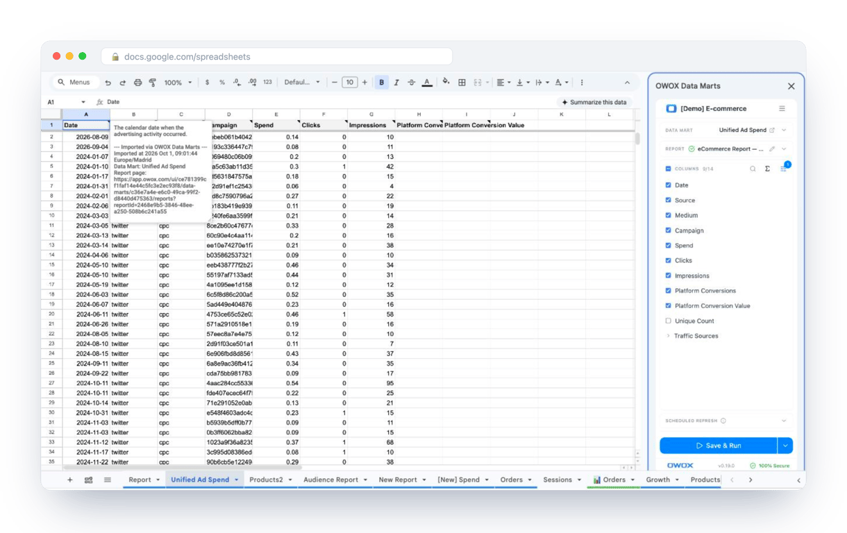
What changes for the person who maintains the sheet:
- Refresh replaces re-export. Refresh current report in the extension menu re-runs the same pull, and a scheduled refresh keeps the tab current without anyone touching it.
- The source is written on the sheet. The header cell of an imported tab carries a note with the data mart it came from, the time of the import and a link to the report.
- No SQL and no warehouse access needed. The analyst decides which data marts and columns are available. You choose from that list.
The extension does not write or change the analyst’s SQL. The conversion from text and timestamps is then written once in that SQL instead of in every sheet, and the date functions here are left for calculations. The extension comes with the OWOX Cloud plans of OWOX Data Marts; spreadsheet reporting describes both ways data reaches a sheet.
Turn your data into decisions.
Governed data marts give you the clean foundation ML needs to actually work.
- No AI hallucinations
- Analyst-governed definitions
- Every number traces to SQL
Frequently Asked Questions
What is the EPOCHTODATE function?
EPOCHTODATE converts a Unix timestamp, the time elapsed since 1 January 1970 00:00 UTC, into a date and time. The syntax is EPOCHTODATE(timestamp, [unit]): unit 1, the default, reads the timestamp as seconds, 2 as milliseconds and 3 as microseconds. For example, EPOCHTODATE(1579046400) returns 15 January 2020, 00:00. The result is in UTC.
What is the EDATE function for?
The EDATE function is used to add or subtract a specific number of months from a given date. The syntax is:=EDATE(start_date, number_of_months)For example,=EDATE(A1, 3)It will calculate the date that is three months after the date in cell A1. It helps calculate future or past dates based on months.
Can I convert text to a date format?
Yes, you can convert text to a date format in Google Sheets by using the DATEVALUE function. This function takes a text string and converts it to a date. For example:=DATEVALUE("2024-09-15")It will convert the string "2024-09-15" into a date value
How do I calculate the number of days between two dates in Google Sheets?
You can use the DATEDIF function to calculate the number of days between two dates. The syntax is:=DATEDIF(start_date, end_date, "D")Here, "D" stands for days. For example: =DATEDIF(A1, B1, "D")It will return the number of days between the dates in cells A1 and B1.