MONTH and EOMONTH functions in Google Sheets: formulas and examples
MONTH returns the month of a date as a number from 1 to 12, and EOMONTH returns the last day of a month a given number of months away. This guide covers both, with formulas for the month name, the first and last day of a month, the number of days in it, due dates and monthly totals.

=MONTH(date) returns the month of a date as a number from 1 to 12. =EOMONTH(start_date, months) returns the last day of the month that is a given number of months before or after a date. With February 15, 2023 in cell B3:
| You need | Formula | Result |
|---|---|---|
| Month number | =MONTH(B3) |
2 |
| Month name | =TEXT(B3, "mmmm") |
February |
| Last day of the month | =EOMONTH(B3, 0) |
February 28, 2023 |
| First day of the month | =EOMONTH(B3, -1) + 1 |
February 1, 2023 |
| Number of days in the month | =DAY(EOMONTH(B3, 0)) |
28 |
| Last day of the next month | =EOMONTH(B3, 1) |
March 31, 2023 |
MONTH function
Syntax of MONTH
=MONTH(date)
- date: the date to take the month from. It can be a cell with a date, a function that returns a date, such as DATE(2024, 11, 15), or a date typed in quotes in a format your spreadsheet locale recognizes.
The result is a number: 1 for January, 12 for December.
Examples of MONTH
The most common form takes the date from a cell:
=MONTH(B3)
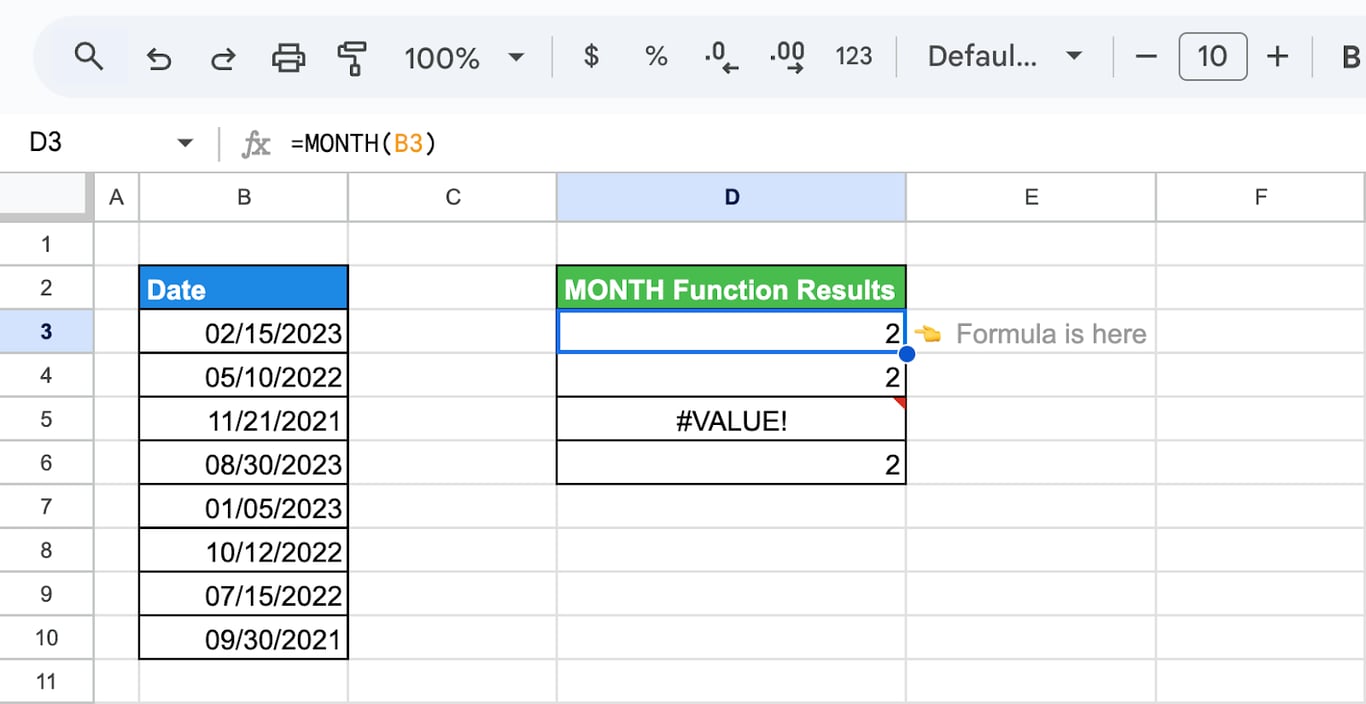
B3 holds February 15, 2023, and the function returns 2.
A date can also be typed into the formula:
=MONTH("2/15/2023")
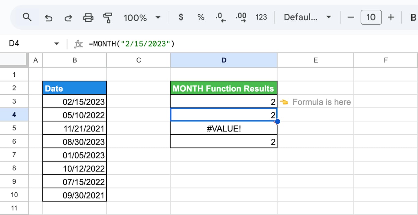
Sheets reads the text as a date in the format of the spreadsheet locale. In a United States locale “2/15/2023” is February 15; the same string written day first, “15/2/2023”, returns #VALUE! there. DATE(2023, 2, 15) means the same in every locale.
A month name on its own is not a date:
=MONTH("February")
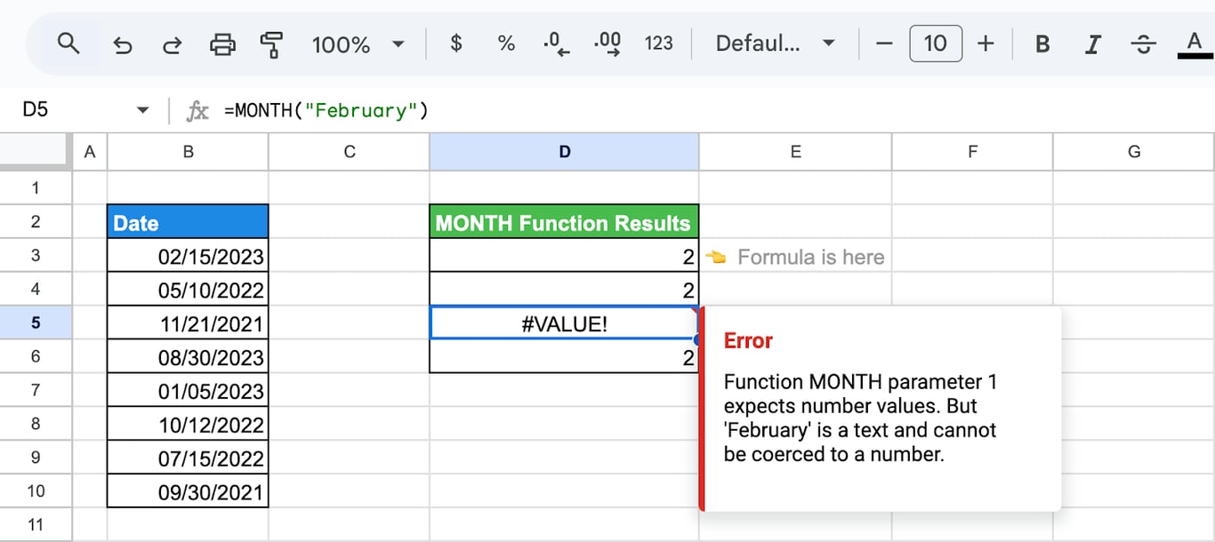
The function returns #VALUE!, and the message says that ‘February’ is text and cannot be coerced to a number.
A month and a day are enough:
=MONTH("February 15")
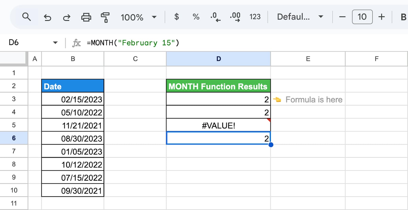
Sheets fills in the current year and reads the text as a date, so the result is 2.
EOMONTH function
Syntax of EOMONTH
=EOMONTH(start_date, months)
- start_date: the date to count from.
- months: the number of months to move. 0 stays in the month of the start date, a positive number moves forward, a negative number moves back. Decimals are cut off, so 1.9 is treated as 1.
The result is always the last day of the month the function lands in, whatever the day of the start date.
Examples of EOMONTH
A positive number moves forward:
=EOMONTH(B3, 2)
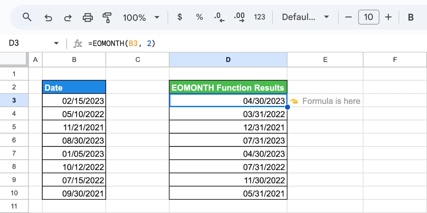
From February 15, 2023 the function moves two months forward and returns April 30, 2023.
A negative number moves back:
=EOMONTH(B4, -2)
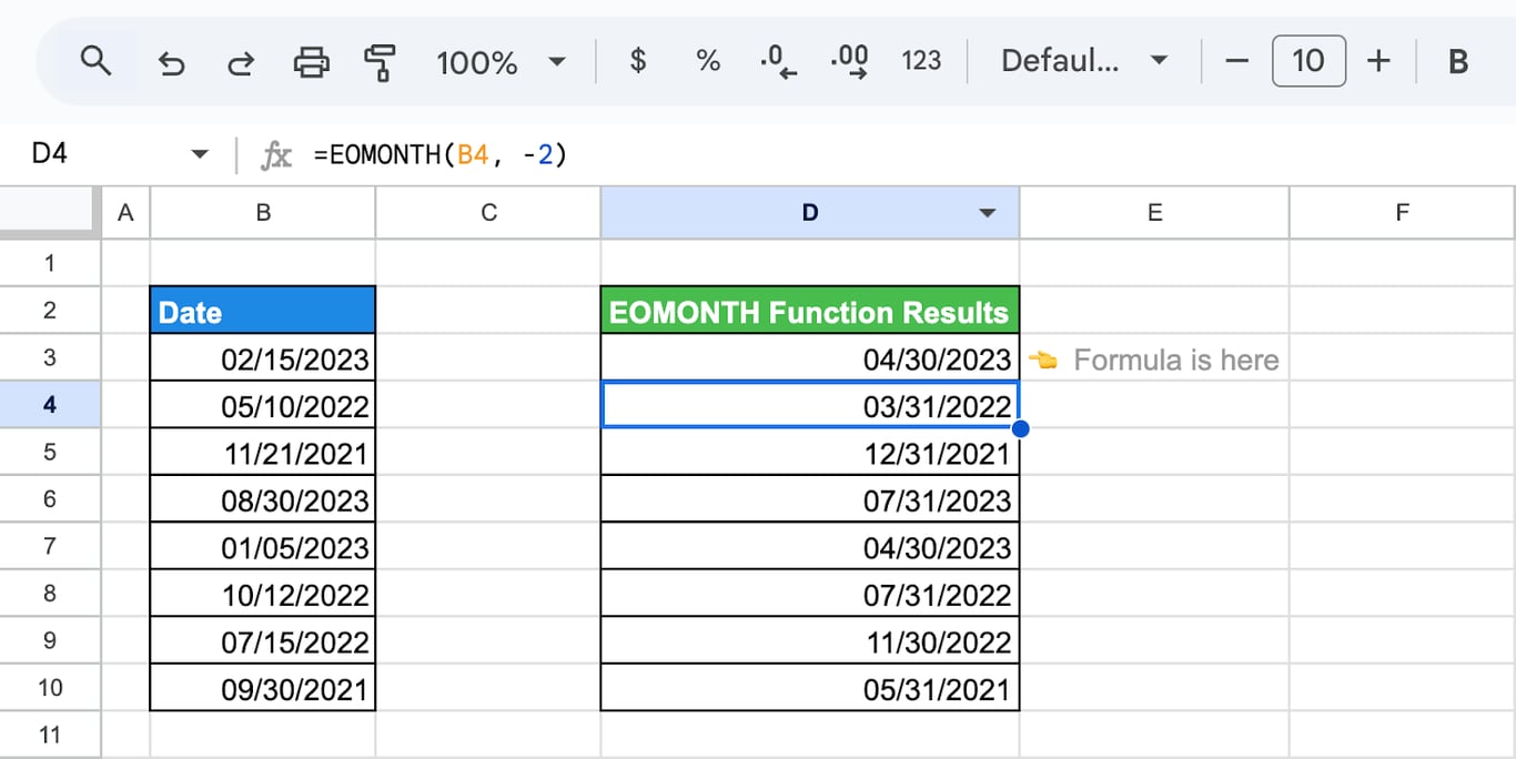
From May 10, 2022 the function moves two months back and returns March 31, 2022.
OWOX Data Marts
See your first report built in real time. 15 minutes.
- Connect your data warehouse
- Pick your metrics
- Get a live Google Sheets report
In the time it takes to write a ticket. Then imagine never writing that ticket again.
Book a DemoWe'll use your actual use case
Practical examples with EOMONTH
Practical examples with EOMONTH
Last day of the month
=EOMONTH(B3, 0)
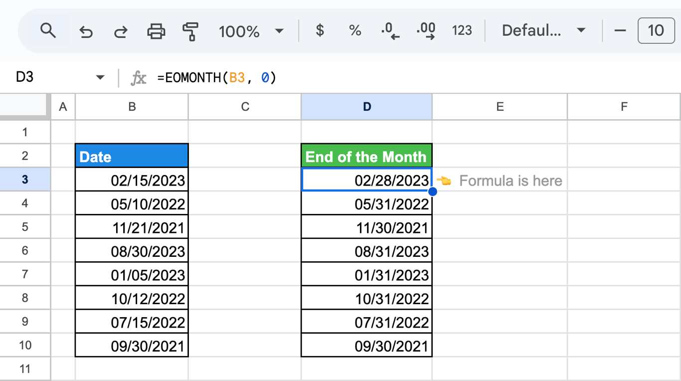
With 0 as the second argument the function returns the last day of the month of the date itself. The result is a convenient label for grouping: every date of the same month gets the same value, and months of different years stay apart.
First day of the month
There is no “start of month” function. Take the last day of the previous month and add one day:
=EOMONTH(B3, -1) + 1
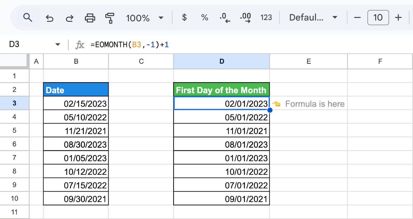
To convert a whole column at once, wrap the formula in ARRAYFORMULA and pass the range:
=ARRAYFORMULA(EOMONTH(B3:B10, -1) + 1)
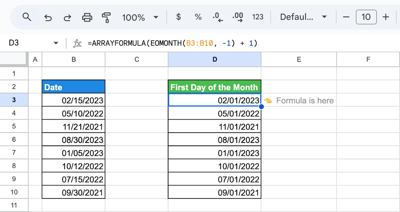
One formula in D3 fills the column down to D10.
Last day of the current month
TODAY returns the current date, so this formula moves on by itself when a new month starts:
=EOMONTH(TODAY(), 0)
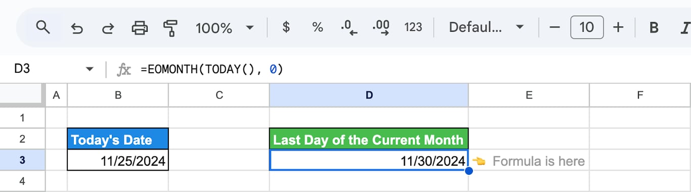
=EOMONTH(TODAY(), 0) - TODAY() gives the number of days left in the month.
Number of days in a month
DAY returns the day of the month. Applied to the last day of a month, it returns the length of that month:
=DAY(EOMONTH(B3, 0))
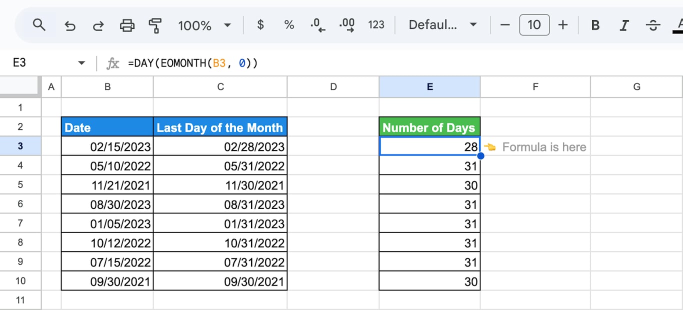
The formula returns 28 for February 2023 and takes leap years into account: for a date in February 2024 it returns 29.
Due dates
For a payment term counted from the end of the month, add the number of days to the month end:
=EOMONTH(B3, 0) + 30
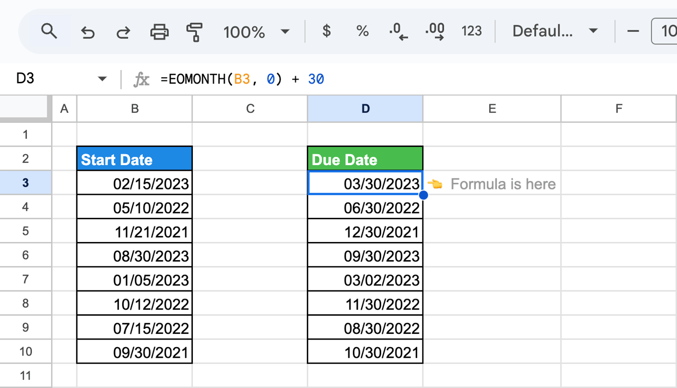
An invoice dated February 15, 2023 with “30 days end of month” terms is due on March 30, 2023. For “end of the following month”, use =EOMONTH(B3, 1).
Eligibility dates
When a period is counted in whole calendar months, the day of the start date does not matter, and EOMONTH gives the date directly:
=EOMONTH(C3, 3)
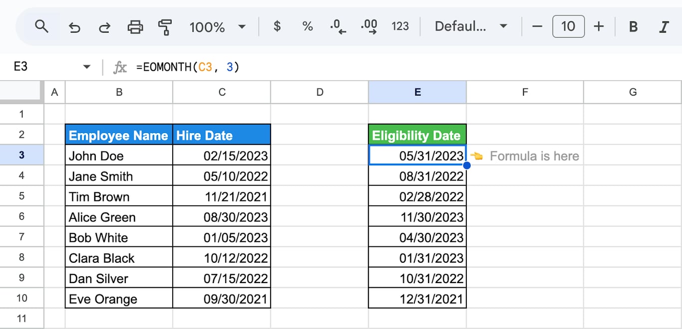
An employee hired on February 15, 2023 becomes eligible at the end of the third month after the hire month, May 31, 2023.
Last day of a month from a month number
When the sheet holds month numbers and not dates, build the first day of the month with DATE and pass it to EOMONTH:
=EOMONTH(DATE(2023, B3, 1), 0)
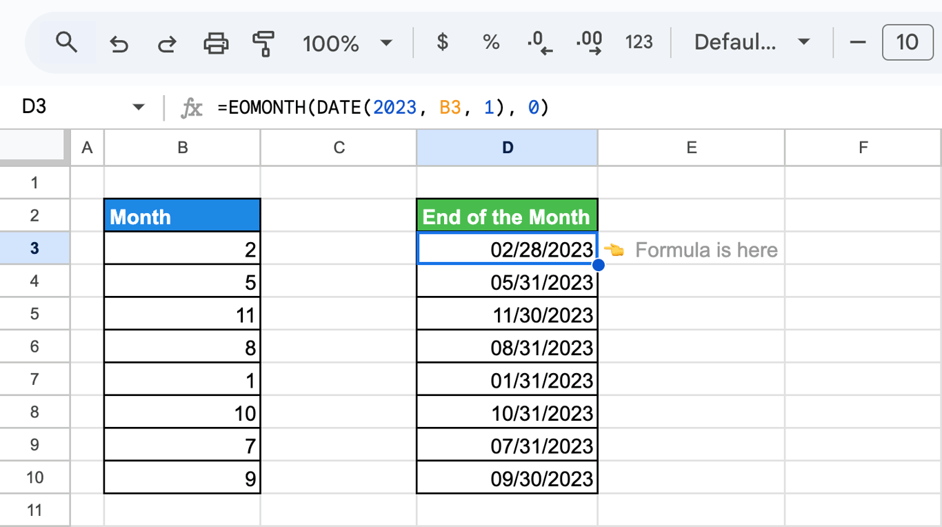
Last Monday of the month
WEEKDAY with 2 as the second argument numbers the days from Monday (1) to Sunday (7). Subtract that number from the last day of the month and add 1 to land on the Monday of the same week:
=EOMONTH(B3, 0) - WEEKDAY(EOMONTH(B3, 0), 2) + 1
- EOMONTH(B3, 0): the last day of the month.
- WEEKDAY(EOMONTH(B3, 0), 2): the day of the week of that date, 1 for Monday to 7 for Sunday.
- + 1: moves from the Sunday before that week to its Monday.
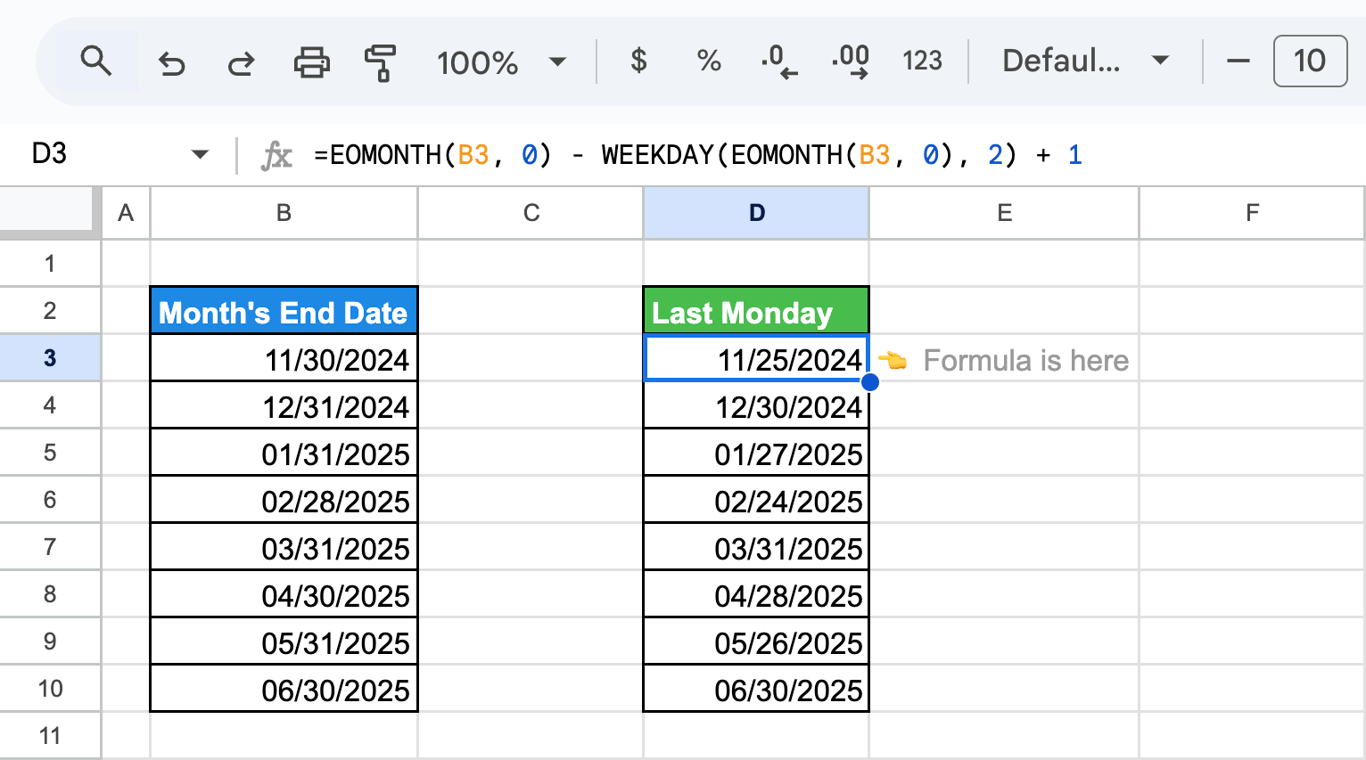
November 30, 2024 is a Saturday, day 6, so the formula returns November 25. When the month ends on a Monday, as March 2025 does, the result is the last day itself.
MONTH and EOMONTH with other functions
MONTH and EOMONTH with other functions
Month name from a date
The shortest way is the TEXT function: =TEXT(B3, "mmmm") returns February, =TEXT(B3, "mmm") returns Feb and =TEXT(B3, "mmmm yyyy") returns February 2023. TEXT writes the name in the language of the spreadsheet locale.
For names of your own, for example in another language or abbreviated your way, use CHOOSE with MONTH as the index:
=CHOOSE(MONTH(B3), "January", "February", "March", "April", "May", "June", "July", "August", "September", "October", "November", "December")
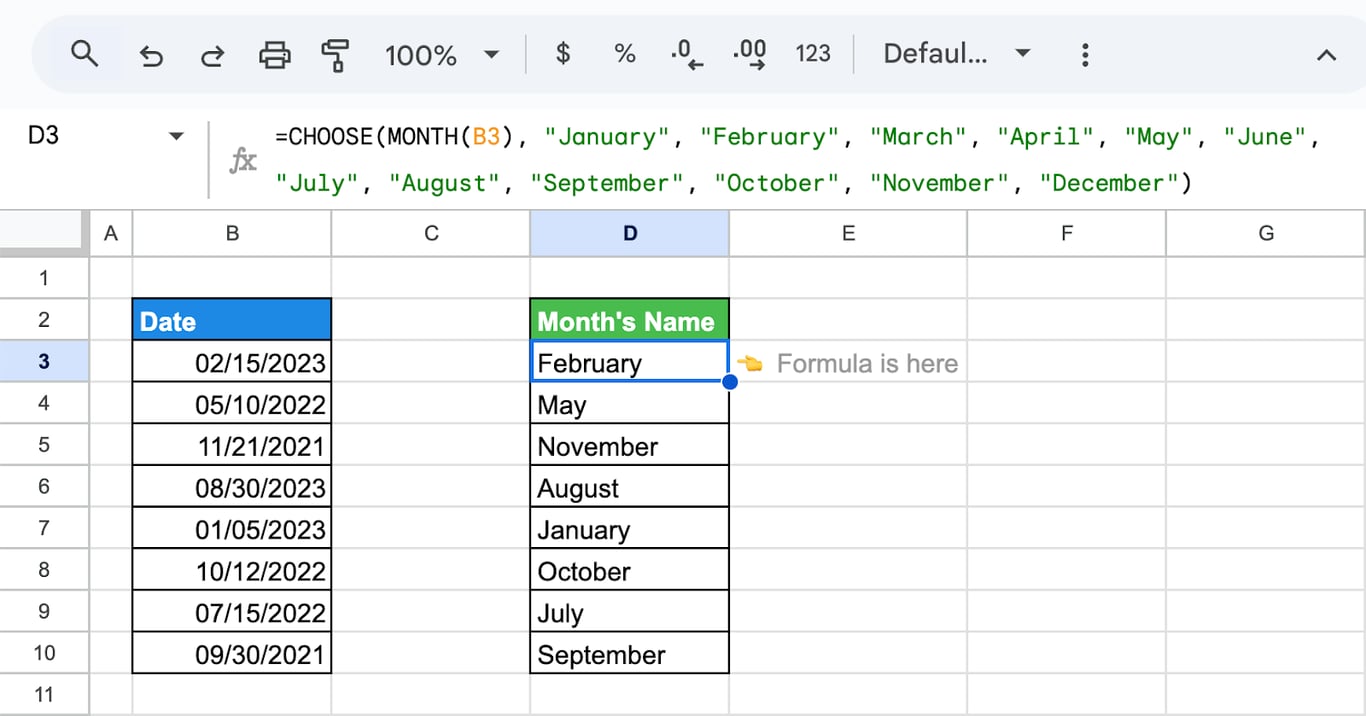
MONTH returns the position, and CHOOSE returns the item at that position in the list.
Monthly totals with SUMIFS
SUMIFS cannot take MONTH(range) as a criteria range: =SUMIFS(C3:C10, MONTH(B3:B10), 1) returns #VALUE!. There are two ways around it.
A helper column. Put =MONTH(B3) next to each row, then sum by that column:
=SUMIFS(C$3:C$10, D$3:D$10, D3)
- C$3:C$10: the amounts to add up.
- D$3:D$10: the helper column with month numbers.
- D3: the month of the current row.
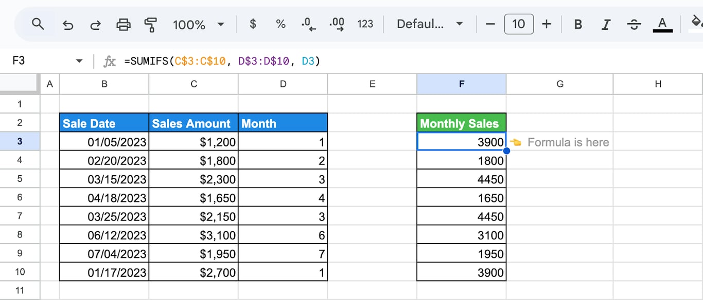
A month number does not know its year: January 2023 and January 2024 would be added together. When the data covers more than one year, use =EOMONTH(B3, 0) as the helper column instead.
A date range. Without a helper column, give SUMIFS the first and the last day of the month. With the first day of the month in F3:
=SUMIFS(C$3:C$10, B$3:B$10, ">=" & F3, B$3:B$10, "<=" & EOMONTH(F3, 0))
More on these conditions in the guide to SUM, SUMIF and SUMIFS.
A condition on the month with IF
=IF(MONTH(B3)=1, "January Sale", "Other")
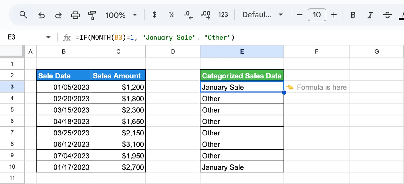
IF checks whether the month of the date is 1 and returns one label for January and another for every other month.
Year, month and day in separate columns
When the three parts sit in separate cells, DATE joins them into a date, and any date function can then work with it:
=MONTH(DATE(B3, C3, D3))
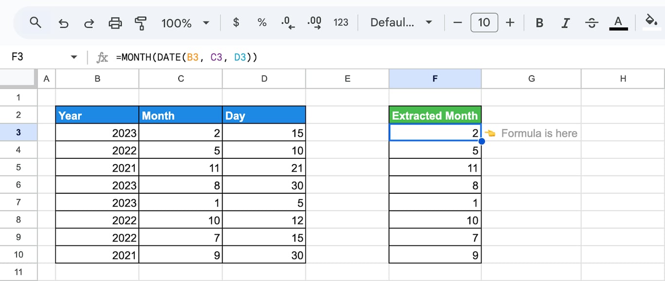
DATE also normalizes values that run over: month 14 of 2023 becomes February 2024, and MONTH returns 2.
Errors and unexpected results
⚠️ Error: #VALUE! in MONTH or EOMONTH.
✅ Solution: The argument is text that Sheets cannot read as a date: a month name alone, a date in the day and month order of another locale, or a date imported as text. Build the date with DATE(year, month, day), or convert the text with DATEVALUE.
⚠️ Error: MONTH returns 12 for an empty cell.
✅ Solution: An empty cell counts as 0, and day 0 in Sheets is December 30, 1899. Skip the blanks: =IF(B3="", "", MONTH(B3)).
⚠️ Error: EOMONTH shows a number such as 44985.
✅ Solution: That is the date as a serial number. Select the cell and choose Format > Number > Date.
⚠️ Error: The year is wrong for a date typed without a year.
✅ Solution: “February 15” is read as February 15 of the current year. Add the year to the text or use DATE.
⚠️ Error: SUMIFS or COUNTIFS returns #VALUE! with MONTH inside.
✅ Solution: These functions need a real range as the criteria range. Use a helper column or a date range, as in the monthly totals example above.
Related Google Sheets functions
Related Google Sheets functions
Functions that are often used next to MONTH and EOMONTH, each with its own guide:
- DATE functions: DATE, EDATE, DATEVALUE and DATEDIF for building and comparing dates.
- YEAR and YEARFRAC: The year of a date and the fraction of a year between two dates.
- DAY, DAYS and DAYS360: The day of the month and the number of days between dates.
- WEEKDAY and WEEKNUM: The day of the week and the week number.
- WORKDAY and NETWORKDAYS: Working days between dates and deadlines in working days.
- QUERY date filtering: Filters rows by a date or a date range inside a QUERY formula.
- Dates and times: Covers formatting, combining, splitting and sorting date and time values.
- Pivot tables: Group dates by month without a formula.
Monthly totals depend on where the rows come from
Monthly totals depend on where the rows come from
MONTH and EOMONTH turn dates into months. What they group is a list of transactions, and in a monthly report that list is the weak point: someone exports last month from a CRM or an ad platform, pastes it under the previous one, and hopes that no row is missing or pasted twice. The month formulas work on whatever is in the tab.
The OWOX Data Marts extension for Google Sheets covers that half. A data analyst publishes a data mart (a table or an SQL query in your data warehouse) and makes it available for reports. In Sheets you open the extension, pick the data mart, tick the columns you want and run it. The rows land in a tab, ready for your formulas.
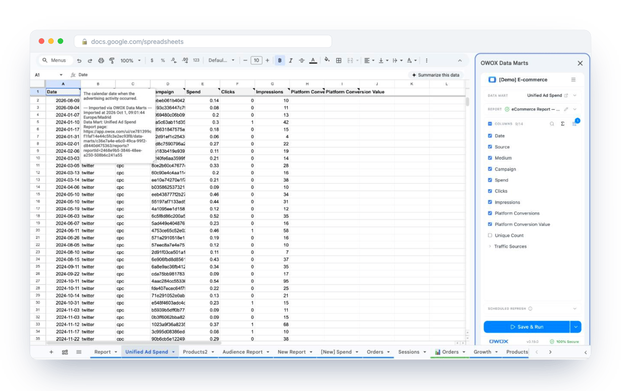
What changes for the person who maintains the sheet:
- Refresh replaces re-export. Refresh current report in the extension menu re-runs the same pull, and a scheduled refresh keeps the tab current without anyone touching it.
- The source is written on the sheet. The header cell of an imported tab carries a note with the data mart it came from, the time of the import and a link to the report.
- No SQL and no warehouse access needed. The analyst decides which data marts and columns are available. You choose from that list.
The extension does not write or change the analyst’s SQL. The monthly formulas stay in the sheet; the rows they add up come from the same data mart on every refresh. The extension comes with the OWOX Cloud plans of OWOX Data Marts; spreadsheet reporting describes both ways data reaches a sheet.
Turn your data into decisions.
Governed data marts give you the clean foundation ML needs to actually work.
- No AI hallucinations
- Analyst-governed definitions
- Every number traces to SQL
Frequently Asked Questions
Can I combine MONTH or EOMONTH with other functions like SUMIFS or IF?
Yes, with one limit: SUMIFS cannot take MONTH(range) as a criteria range and returns #VALUE!. Add a helper column with =MONTH(B3) and sum by it, or give SUMIFS a date range: =SUMIFS(C:C, B:B, ">=" & F3, B:B, "<=" & EOMONTH(F3, 0)), where F3 holds the first day of the month. Inside IF, MONTH works directly: =IF(MONTH(B3)=1, "January", "Other").
How do I calculate the number of days in a month using EOMONTH?
To calculate the number of days in a month, use EOMONTH to find the last day, then subtract the first day. For example, =EOMONTH(A1,0) - EOMONTH(A1,-1) returns the days in the month of the date in A1, including leap years.
What happens if I get a #VALUE! error in EOMONTH?
A #VALUE! error in EOMONTH usually occurs if the date argument is invalid or not formatted correctly. Ensure you provide a valid date or a cell with a date. For text dates, try using DATE or DATEVALUE to convert them before using EOMONTH.
Can I use the MONTH function to display month names instead of numbers?
Yes, to display month names with the MONTH function, combine it with the TEXT function.For example, use =TEXT(A1, "MMMM") to show the full month name (e.g., "January") or =TEXT(A1, "MMM") for the abbreviated name (e.g., "Jan"), where A1 contains a date.
What is the difference between EOMONTH and MONTH in Google Sheets?
The MONTH function returns the month number (1–12) of a specific date, while EOMONTH returns the last day of the month, either in the current month or a specified number of months before or after. Use EOMONTH for end-of-month calculations.
How does the MONTH function work in Google Sheets?
The MONTH function in Google Sheets extracts the month from a given date and returns it as a number between 1 (January) and 12 (December). Use it by typing =MONTH(date), where "date" is a valid date or cell reference containing a date.