SORT and SORTN in Google Sheets: syntax, top N and ties
SORT returns a sorted copy of a range, by one or several columns, and leaves the source untouched. SORTN returns only the first N rows of the sorted result and has four modes for ties and duplicates. This guide shows the syntax of both, sorting by several columns and by a custom order, the tie modes on one example, and the mistakes that return the wrong rows.
SORT returns a sorted copy of a range. SORTN returns only the first rows of that sorted copy.
=SORT(B3:D10, 3, FALSE)
=SORTN(B3:D10, 3, 0, 3, FALSE)
The first formula returns all rows of B3:D10, ordered by the third column from the largest value down. The second returns the top three of them. Neither changes the source: the result appears next to it and updates when the data changes.
SORT
=SORT(range, sort_column, is_ascending, [sort_column2, is_ascending2, ...])
- range: the data to sort, without its header row.
- sort_column: the number of the column inside the range to sort by, or a separate range of the same height.
- is_ascending: TRUE for A to Z and smallest first, FALSE for the reverse.
- More pairs of column and direction break ties in the order they are listed.
With the range alone, =SORT(B3:B10), the result is sorted by the first column in ascending order.
=SORT(B3:D10, 3, TRUE)
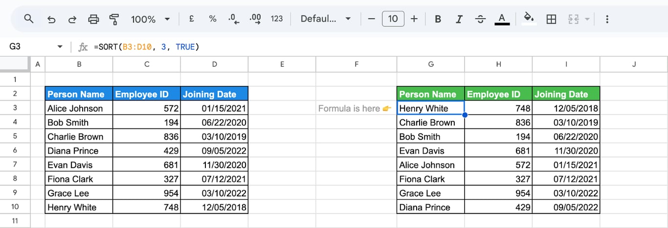
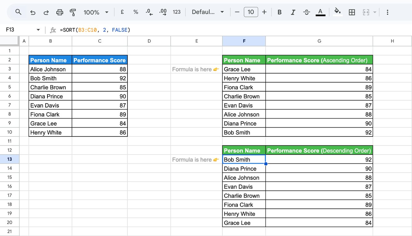
Ascending and descending
=SORT(B3:C10, 2, TRUE)
=SORT(B3:C10, 2, FALSE)
Several columns
=SORT(B3:C10, 2, TRUE, 1, TRUE)
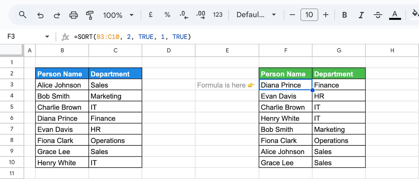
The first pair is the main order, the second decides between rows that are equal in the first.
Sort by a range, also one outside the data
The sort column can be a range instead of a number. That makes the formula independent of the column’s position, and allows sorting by a column that is not part of the output:
=SORT(C3:C10, B3:B10, FALSE)
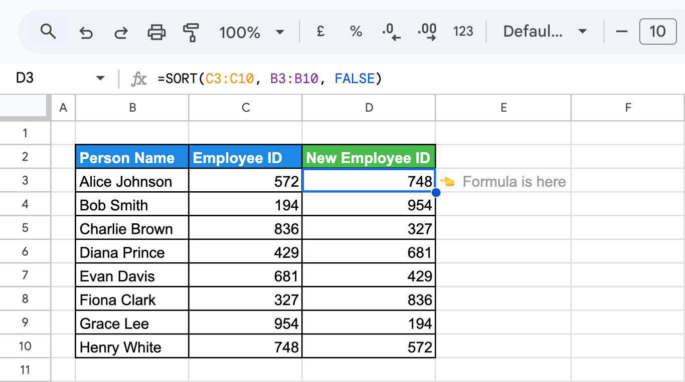
The same form sorts by a calculated value. For a custom order that is not alphabetical, sort by the position of each value in a list:
=SORT(B3:D10, MATCH(C3:C10, {"High"; "Medium"; "Low"}, 0), TRUE)
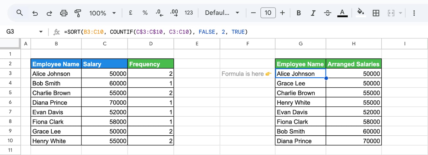
MATCH returns 1 for “High”, 2 for “Medium” and 3 for “Low”, and SORT orders the rows by those numbers. And for most frequent values first:
=SORT(B3:C10, COUNTIF(C$3:C$10, C3:C10), FALSE, 2, TRUE)
Data from another tab, open-ended ranges
=SORT(Dataset!B3:E, 3, TRUE)
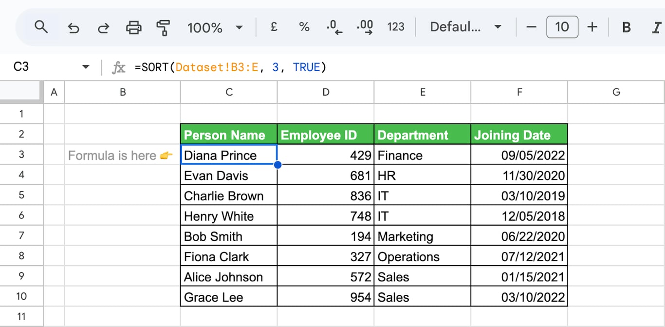
A range without an end row, B3:E, includes rows added later. It also includes the empty rows below the data; wrap the range in FILTER to keep them out of the result: =SORT(FILTER(B3:E, B3:B <> ""), 3, FALSE).
How values are ordered
- Numbers come before text, and text before TRUE and FALSE.
- Text is ordered without regard to case.
- Numbers stored as text are sorted as text: “10”, “100”, “9”. Convert them with VALUE first.
SORTN
=SORTN(range, [n], [display_ties_mode], [sort_column, is_ascending, ...])
- n: how many rows to return. 1 if omitted.
- display_ties_mode: what to do with ties and duplicates, a number from 0 to 3.
- sort_column, is_ascending: as in SORT. If omitted, the range is sorted by its first column in ascending order.
=SORTN(B3:D10, 3, 0, 3, FALSE)
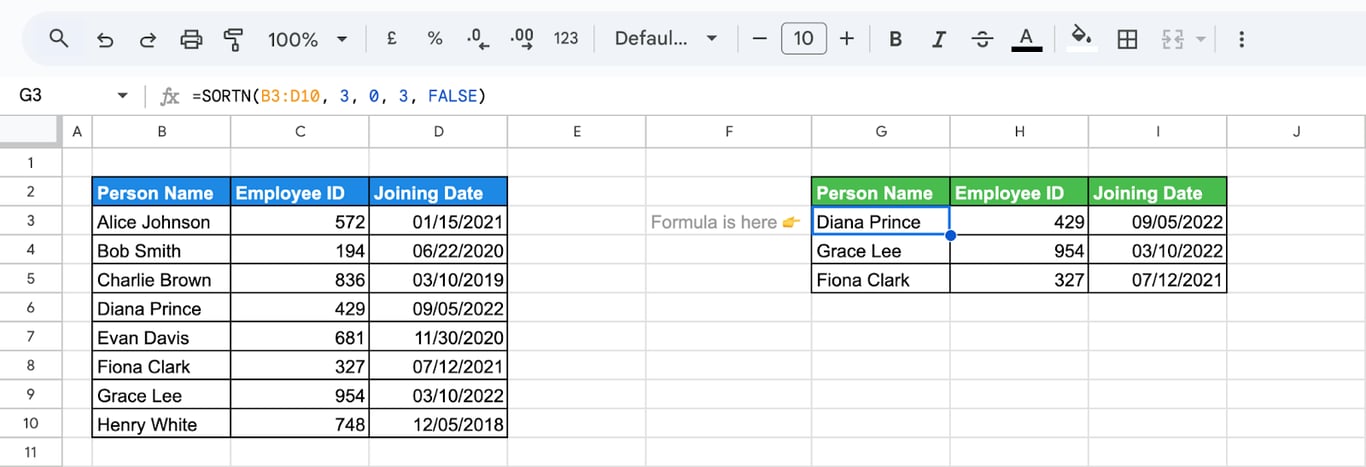
Top and bottom N
=SORTN(B3:C10, 5, 0, 2, FALSE)
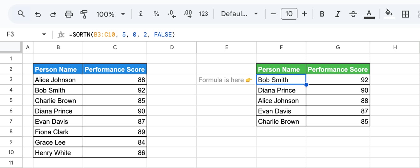
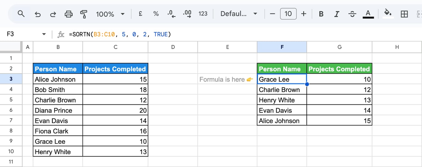
For the bottom five, sort in ascending order:
=SORTN(B3:C10, 5, 0, 2, TRUE)
The four tie modes
The modes differ only when values repeat. In this table two people earn 55,000 and two earn 50,000, and the top of the salary column reads 70,000, 60,000, 58,000, 55,000, 55,000, 52,000.
| Mode | Returns | SORTN(B3:D10, n, mode, 3, FALSE) |
|---|---|---|
| 0 | Exactly n rows | n = 5: 70,000, 60,000, 58,000, 55,000, 55,000 |
| 1 | n rows, plus any rows tied with the last one | n = 4: the same five rows, because the fifth ties with the fourth |
| 2 | n rows after duplicates are removed | n = 5: 70,000, 60,000, 58,000, 55,000, 52,000 |
| 3 | The first n distinct values, with all their duplicates | n = 5: six rows, both 55,000 rows included |
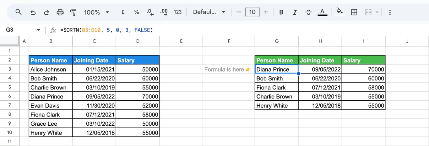
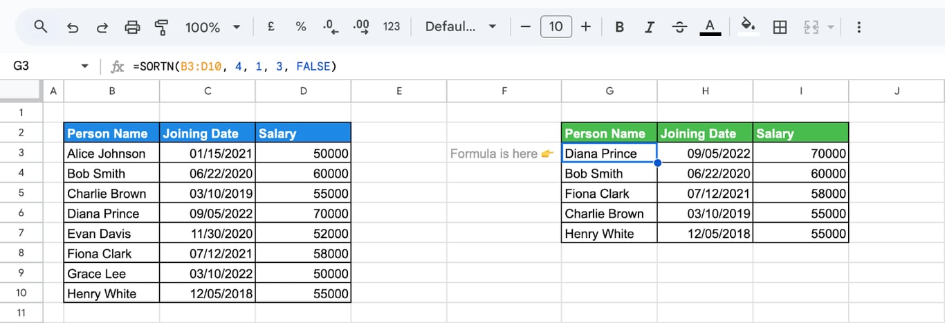
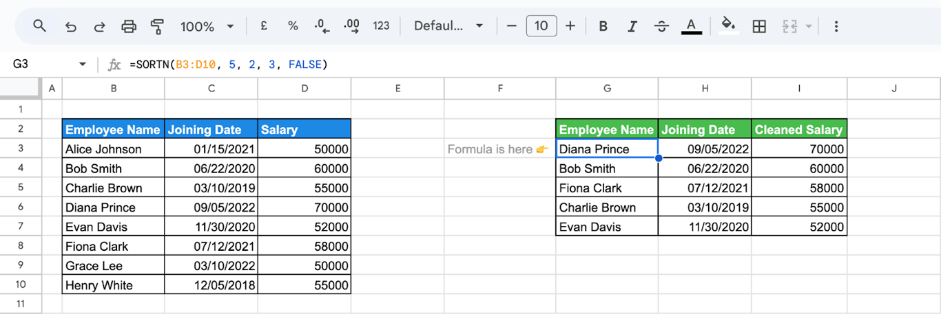
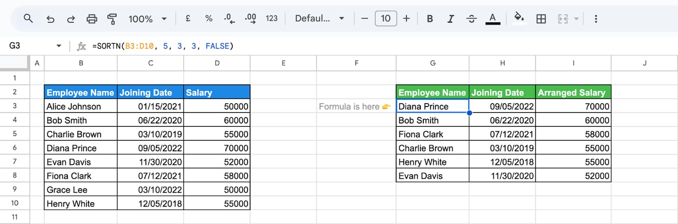
Mode 1 is the fair one for leaderboards: nobody is cut off by a tie. Mode 2 with a large n is a way to remove duplicates by one column: =SORTN(B3:D10, 9^9, 2, 2, TRUE) returns one row for each value of the second column. More ways in the guide to removing duplicates.
The sort column is not optional in practice
Without a sort column, SORTN sorts by the first column of the range in ascending order, whatever order the data had. =SORTN(B3:D10, 3) does not return “the first three rows”: it returns the first three after sorting by column B. A range that is already sorted, for example by a QUERY with ORDER BY, is re-sorted and the top three are lost. Always name the column and the direction.
OWOX Data Marts
See your first report built in real time. 15 minutes.
- Connect your data warehouse
- Pick your metrics
- Get a live Google Sheets report
In the time it takes to write a ticket. Then imagine never writing that ticket again.
Book a DemoWe'll use your actual use case
SORT and SORTN with other functions
SORT and SORTN with other functions
FILTER: sort only the rows you need
=SORT(FILTER(B3:D10, C3:C10="Sales", D3:D10>45000), 3, TRUE, 1, TRUE)
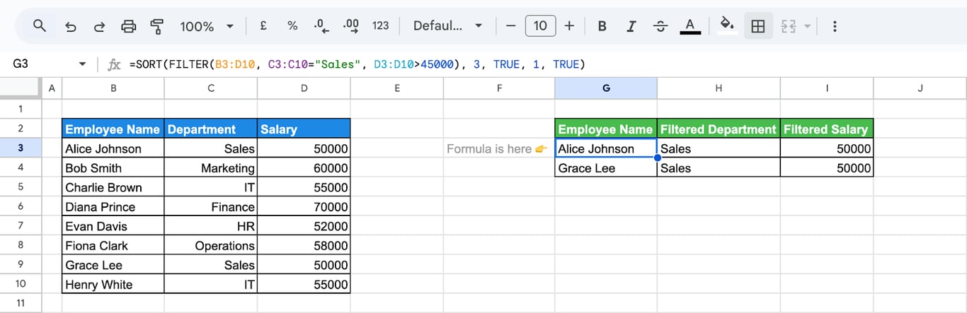
For “either condition”, add the conditions inside FILTER: (C3:C10="Sales") + (D3:D10>55000).
UNIQUE: a sorted list without repeats
=SORT(UNIQUE(D3:D10), 1, TRUE)
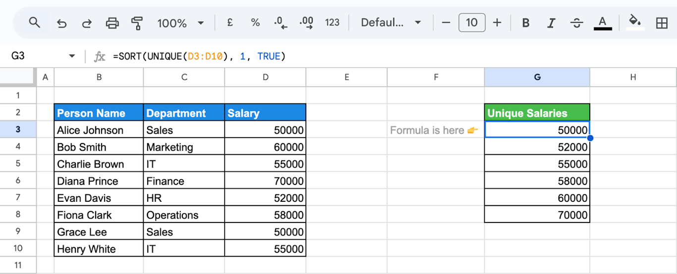
See UNIQUE.
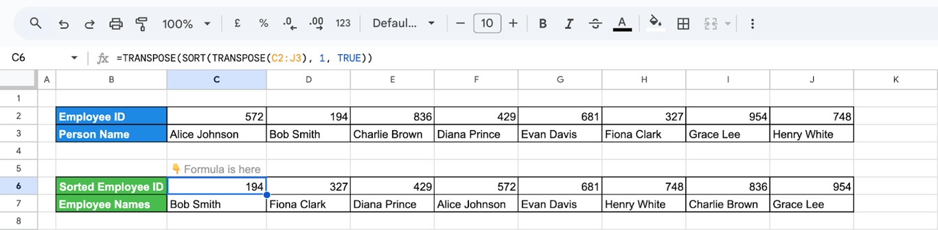
TRANSPOSE: sort data laid out in a row
SORT orders rows. For data that runs across, turn it, sort it and turn it back:
=TRANSPOSE(SORT(TRANSPOSE(C2:J3), 1, TRUE))
QUERY: filter the sorted result
=QUERY(SORT(B3:C10, 2, FALSE), "SELECT * WHERE Col2 >= 55000")
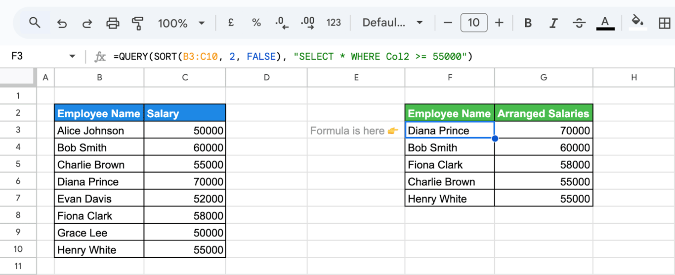
QUERY can do both steps itself with WHERE and ORDER BY; use whichever reads better.
SORT, SORTN or the menu
- Data > Sort range rearranges the cells themselves, once. Use it for a table you maintain by hand. See how to sort data.
- SORT leaves the source alone and stays up to date. Use it for a report built on data that changes.
- SORTN is SORT with a row limit and tie handling. Use it for top lists.
Errors and wrong results
⚠️ Error: #REF! with “Array result was not expanded”.
✅ Solution: The result needs cells that are not empty. Clear the space below and to the right of the formula.
⚠️ Error: An error after a sort column number was typed.
✅ Solution: The number is larger than the number of columns in the range. Columns are counted from the left edge of the range, not of the sheet: in B3:D10, column D is 3.
⚠️ Error: The header row ends up in the middle of the result.
✅ Solution: The range includes the header. Start the range one row lower.
⚠️ Error: Numbers are in the order 10, 100, 9.
✅ Solution: They are stored as text. Convert the column to numbers.
⚠️ Error: Empty rows in the result.
✅ Solution: The range is open-ended and includes the blank rows below the data. Filter them out before sorting.
⚠️ Error: SORTN returns the wrong rows.
✅ Solution: The sort column or direction is missing, so the range was sorted by its first column in ascending order. Add them.
⚠️ Error: SORTN returns more rows than n.
✅ Solution: Tie mode 1 or 3 adds the tied rows. Use mode 0 for an exact count.
Related guides
- How to sort data: Sorting from the menu.
- FILTER: Rows that meet a condition.
- UNIQUE: Distinct values and rows.
- RANK: The position of each value.
- QUERY: Filter, group and sort in one formula.
- Remove duplicates: Including SORTN in mode 2.
- Array formulas: Formulas that return ranges.
A top list is only as complete as its rows
A top list is only as complete as its rows
SORTN gives an exact top five of the rows in the range. If the range is an export that stops at last Tuesday, or lacks one region, the list is exact and wrong, and a ranking is the kind of result people act on: budgets move to the campaigns at the top.
The OWOX Data Marts extension for Google Sheets covers that half. A data analyst publishes a data mart (a table or an SQL query in your data warehouse) and makes it available for reports. In Sheets you open the extension, pick the data mart, tick the columns you want and run it. The rows land in a tab, ready for your formulas.

What changes for the person who maintains the sheet:
- Refresh replaces re-export. Refresh current report in the extension menu re-runs the same pull, and a scheduled refresh keeps the tab current without anyone touching it.
- The source is written on the sheet. The header cell of an imported tab carries a note with the data mart it came from, the time of the import and a link to the report.
- No SQL and no warehouse access needed. The analyst decides which data marts and columns are available. You choose from that list.
The extension does not write or change the analyst’s SQL. SORT and SORTN then rank the complete, current rows on every refresh. The extension comes with the OWOX Cloud plans of OWOX Data Marts; spreadsheet reporting describes both ways data reaches a sheet.
Turn your data into decisions.
Governed data marts give you the clean foundation ML needs to actually work.
- No AI hallucinations
- Analyst-governed definitions
- Every number traces to SQL
Frequently Asked Questions
How can I sort data from another tab in Google Sheets using the SORT function?
To sort data from another tab, reference the tab name in the SORT function. For example, =SORT(Sheet2!A2:C10, 2, TRUE) sorts data from Sheet2, using the second column in ascending order. Replace Sheet2 with the desired tab name and adjust the range and criteria as needed.
What should I do if I encounter a #VALUE! error while using the SORT function?
Check the sort column first: its number is counted from the left edge of the range, so in B3:D10 column D is 3, and a number larger than the range has columns returns an error. A sort range must have the same number of rows as the data. If the error is #REF! with 'Array result was not expanded', the cells where the result should go are not empty.
How do I remove duplicates when sorting data in Google Sheets?
To remove duplicates when sorting data, combine the SORT and UNIQUE functions. For example, use =SORT(UNIQUE(A2:C10), 1, TRUE) to first remove duplicates from the range A2:C10 and then sort the data by the first column in ascending order. This ensures unique, organized results.
Can I sort data by multiple columns in Google Sheets?
Yes, you can sort data by multiple columns using the SORT function. Specify the range and sorting criteria for each column. For example, =SORT(A2:C10, 1, TRUE, 2, FALSE) sorts by the first column in ascending order, then by the second column in descending order, layering sorting logic.
How do I sort data in ascending or descending order using the SORT function?
Use the SORT function to organize data in ascending or descending order by specifying the range, column, and order. For example, =SORT(A2:C10, 2, TRUE) sorts the data by the second column in ascending order. Replace TRUE with FALSE for descending order. This simplifies dynamic data organization.
What is the difference between the SORT and SORTN functions in Google Sheets?
SORT returns all rows of the range in sorted order. SORTN returns only the first n rows of the sorted result and has four modes for ties: 0 returns exactly n rows, 1 adds the rows tied with the last one, 2 removes duplicates first, and 3 returns n distinct values with all their duplicates. Without a sort column SORTN sorts by the first column in ascending order, so always name the column and the direction.