EXACT function in Google Sheets: case-sensitive comparison, lookup and count
EXACT compares two values character by character, including the case of the letters, and returns TRUE or FALSE. The equals sign and most lookup functions ignore case; EXACT is what makes them case-sensitive. This guide covers the syntax, how EXACT differs from the equals sign, case-sensitive XLOOKUP, MATCH, FILTER and counting, and the behaviours worth knowing before relying on it.
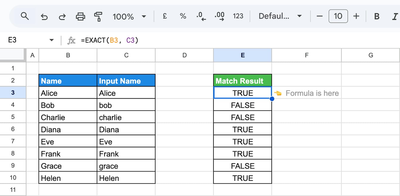
EXACT compares two values and returns TRUE only if they are identical, including the case of the letters:
=EXACT(B3, C3)
“Bob” and “bob” give FALSE. The equals sign, =B3=C3, gives TRUE for the same pair: it ignores case, and so do VLOOKUP, XLOOKUP, MATCH and COUNTIF. EXACT is the way to make a comparison, a lookup or a count case-sensitive.
EXACT syntax
=EXACT(string1, string2)
- string1, string2: the two values to compare: cells, texts in quotes or results of other functions.
The result is TRUE or FALSE.
=EXACT(B3, C3)
EXACT and the equals sign
The results in this table come from our test sheet.
| Comparison | = |
EXACT |
|---|---|---|
| “Google” and “google” | TRUE | FALSE |
| “abc” and “abc “ with a space at the end | FALSE | FALSE |
| The number 123 and the text “123” | FALSE | TRUE |
| The number 1500 and the text “1,500” | FALSE | FALSE |
| An empty cell and “” | TRUE | TRUE |
Three things follow.
- Case is the only extra strictness. Spaces already make two values different for both. Wrap the values in TRIM to ignore them:
=EXACT(TRIM(B3), TRIM(C3)). - EXACT compares as text. A number and the same number stored as text are equal for EXACT and different for the equals sign. That makes EXACT useful for comparing IDs from two exports where one side arrived as text.
- The number format is not compared. A cell that holds 1500 and shows “1,500” equals 1500, not the text “1,500”. A date equals the same date whatever format either cell has.
OWOX Data Marts
See your first report built in real time. 15 minutes.
- Connect your data warehouse
- Pick your metrics
- Get a live Google Sheets report
In the time it takes to write a ticket. Then imagine never writing that ticket again.
Book a DemoWe'll use your actual use case
Compare two columns
=EXACT(C3, D3)
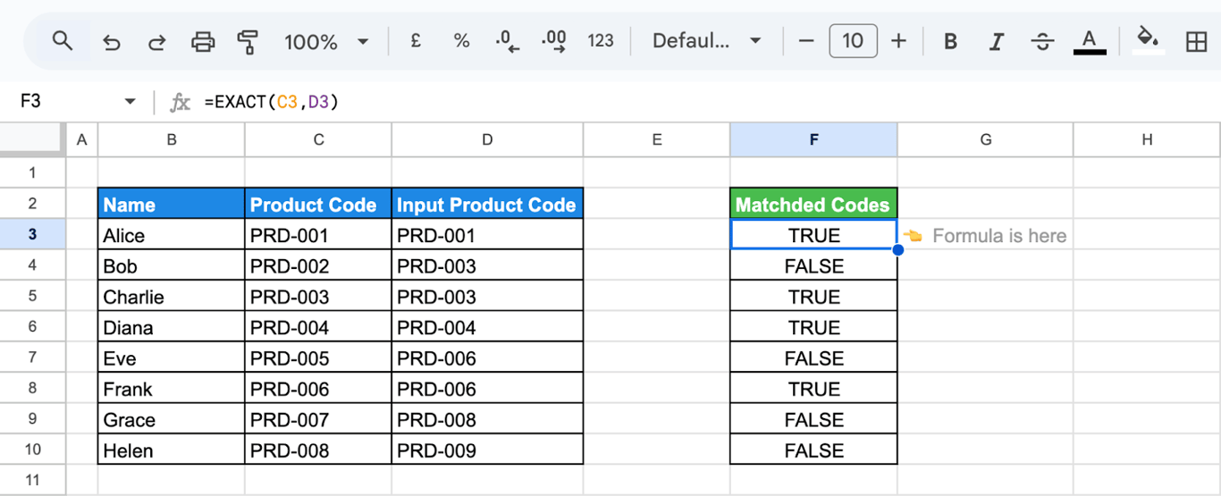
For a whole column from one formula:
=ARRAYFORMULA(EXACT(C3:C10, D3:D10))
Without ARRAYFORMULA a range in EXACT does not expand; in our test it returned #VALUE!.
A label instead of TRUE and FALSE
=IF(EXACT(C3, D3), "Match", "No Match")
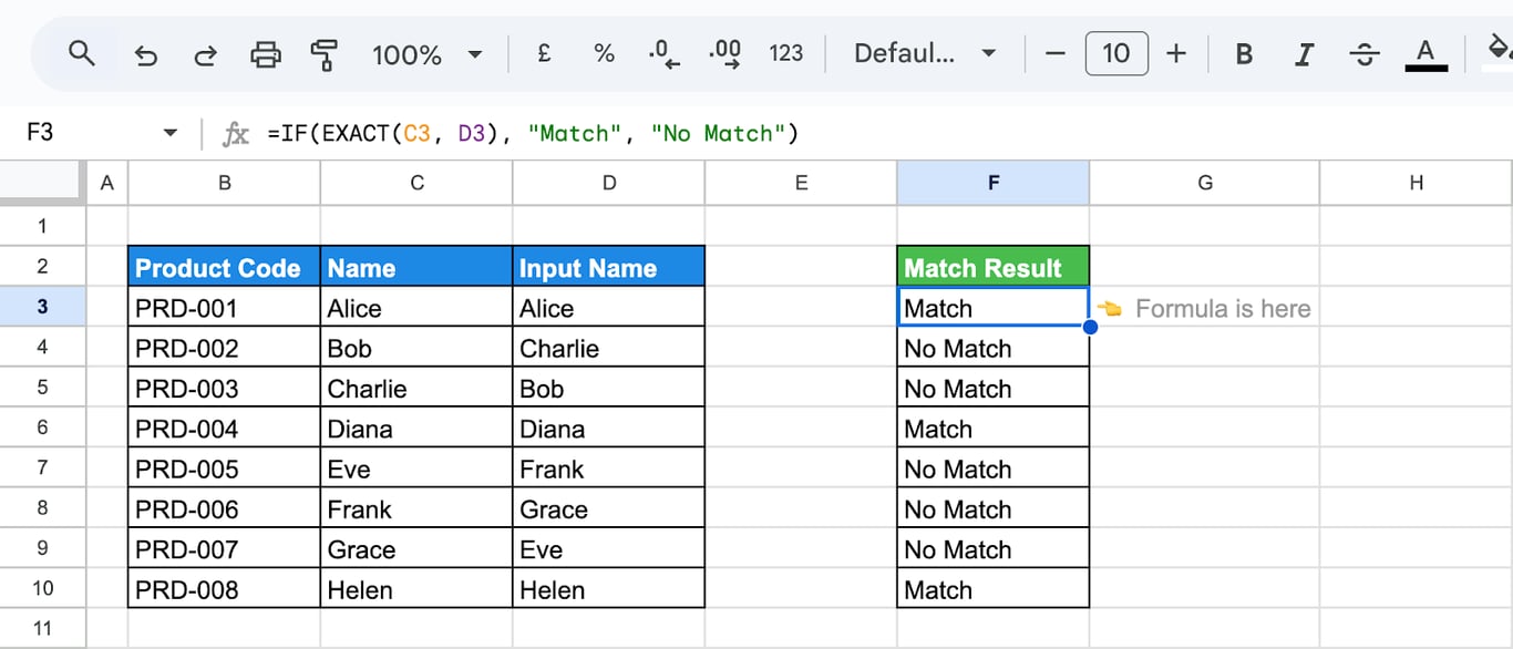
See the IF function.
Skip the rows with a missing value
Two empty cells are equal, so EXACT returns TRUE for them. To mark such rows instead:
=IF(OR(ISBLANK(C3), ISBLANK(D3)), "N/A", EXACT(C3, D3))
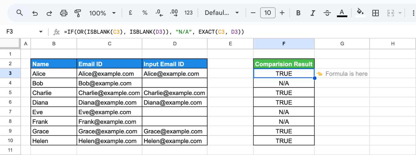
Highlight the differences
In Format > Conditional formatting, choose Custom formula is and enter the comparison for the first row of the range, with the columns fixed:
=NOT(EXACT($C3, $D3))
Rows where the two columns differ, in case or in anything else, get the format.
Case-sensitive lookup
XLOOKUP, VLOOKUP and MATCH find “mike” in a column that holds “Mike”. To make them tell the two apart, look for TRUE in the result of EXACT.
Case-sensitive XLOOKUP
=ARRAYFORMULA(XLOOKUP(TRUE, EXACT(C3:C12, "Mike"), D3:D12))
EXACT compares every cell of C3:C12 with the key and returns a column of TRUE and FALSE; XLOOKUP finds the first TRUE and returns the value from the same row of D3:D12. In our test this returned 3200 for “Mike”. For “mike” it found nothing and returned the fallback text given as a fourth argument, where a plain =XLOOKUP("mike", C3:C12, D3:D12) returned 3200.
ARRAYFORMULA is required: without it the formula returned #N/A or #VALUE!, because EXACT then compares a single cell. More on the function in XLOOKUP and VLOOKUP.
Case-sensitive MATCH and INDEX
=INDEX(D3:D12, MATCH(TRUE, EXACT(C3:C12, "Mike"), 0))
The same idea with MATCH. MATCH alone returns the position of the row.
Check a looked-up value
EXACT also verifies what a lookup returns. Here VLOOKUP finds the name for a product code, and EXACT compares it with the name in the second list:
=EXACT(VLOOKUP(E3, $B$3:$C$10, 2, FALSE), F3)
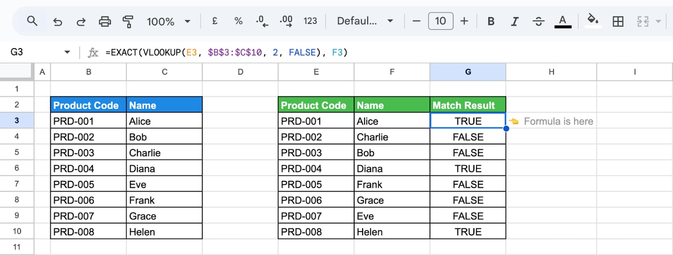
All matching rows
=FILTER(D3:D12, EXACT(C3:C12, "John"))
FILTER returns every row where EXACT is TRUE.
Case-sensitive count and sum
COUNTIF and SUMIF ignore case: in our test =COUNTIF(C3:C12, "sarah") counted the four rows with “Sarah”. With EXACT inside SUMPRODUCT, the case matters:
=SUMPRODUCT(--EXACT(C3:C12, "Sarah"))
returned 4, and the same formula with “sarah” returned 0. The two minus signs turn TRUE and FALSE into 1 and 0. To sum instead of count, multiply by the column of numbers:
=SUMPRODUCT(EXACT(C3:C12, "Sarah") * D3:D12)
See COUNTIF and COUNTIFS for the counts that ignore case.
Check how a value is written
Compared with a changed copy of itself, a value shows whether it follows a rule:
=EXACT(C3, UPPER(C3))is TRUE when the text has no lower-case letters.=EXACT(C3, TRIM(C3))is TRUE when it has no extra spaces.=EXACT(C3, PROPER(C3))is TRUE when every word starts with a capital.
The same formulas work as custom formulas in data validation, to reject entries that break the rule. See also UPPER, LOWER and PROPER.
Problems and fixes
⚠️ Problem: FALSE for two values that look identical.
✅ Solution: One of them has a space at the end or an invisible character. Compare =LEN(C3) and =LEN(D3); if they differ, clean both with TRIM.
⚠️ Problem: TRUE for rows where both cells are empty.
✅ Solution: Empty equals empty. Test for blanks first with ISBLANK.
⚠️ Problem: #VALUE! with a range.
✅ Solution: EXACT compares one pair of values. Wrap the formula in ARRAYFORMULA.
⚠️ Problem: #N/A from the case-sensitive XLOOKUP.
✅ Solution: Either ARRAYFORMULA is missing, or no row matches with this exact case. Add a fourth argument to XLOOKUP for the second situation.
⚠️ Problem: The comparison should ignore case.
✅ Solution: Use the equals sign: =C3=D3.
Related Google Sheets functions
Related Google Sheets functions
- FIND and SEARCH: FIND is the case-sensitive one of the pair.
- MATCH: The position of a value in a range.
- XLOOKUP and VLOOKUP: Lookups, case-insensitive by default.
- IF: Turn TRUE and FALSE into labels.
- TRIM, CLEAN and T: Remove the spaces that break a match.
- Remove duplicates: Duplicates with and without case.
Two lists that have to be compared should not have diverged
Two lists that have to be compared should not have diverged
A column of EXACT formulas between two lists is a reconciliation: the same codes or names were typed or exported twice and may no longer agree. The check finds the differences in this pair of lists; it does not stop the next pair from drifting.
The OWOX Data Marts extension for Google Sheets covers that half. A data analyst publishes a data mart (a table or an SQL query in your data warehouse) and makes it available for reports. In Sheets you open the extension, pick the data mart, tick the columns you want and run it. The rows land in a tab, ready for your formulas.
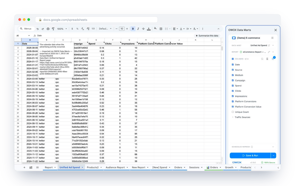
What changes for the person who maintains the sheet:
- Refresh replaces re-export. Refresh current report in the extension menu re-runs the same pull, and a scheduled refresh keeps the tab current without anyone touching it.
- The source is written on the sheet. The header cell of an imported tab carries a note with the data mart it came from, the time of the import and a link to the report.
- No SQL and no warehouse access needed. The analyst decides which data marts and columns are available. You choose from that list.
The extension does not write or change the analyst’s SQL. When both reports are built on the same data mart, their keys are the same values by construction, and EXACT is left for checking what people enter by hand. The extension comes with the OWOX Cloud plans of OWOX Data Marts; spreadsheet reporting describes both ways data reaches a sheet.
Turn your data into decisions.
Governed data marts give you the clean foundation ML needs to actually work.
- No AI hallucinations
- Analyst-governed definitions
- Every number traces to SQL
Frequently Asked Questions
How can I use EXACT for data validation?
You can use the EXACT function with IF to flag mismatches, such as =IF(EXACT(A1, B1), "Valid", "Invalid"). Alternatively, apply it in Conditional Formatting to highlight matching or mismatching cells, ensuring consistency across your dataset. This helps streamline data validation processes effectively.
Can EXACT compare numbers as well as text?
Yes. EXACT compares the values as text, so the number 123 and the text 123 are equal for EXACT, while the equals sign treats them as different. The number format is not part of the comparison: a cell that holds 1500 and displays 1,500 equals 1500, not the text 1,500.
Is the EXACT function case-sensitive?
Yes, the EXACT function is case-sensitive. It distinguishes between uppercase and lowercase letters. For example, "Google" and "google" would not match because of the difference in capitalization. This feature is helpful for tasks requiring strict text comparisons.
How does the EXACT function work in text comparison?
EXACT compares two values character by character, including the case of the letters and any spaces. If every character is the same it returns TRUE, otherwise FALSE. Cell formatting such as colour, font or number format is not compared.
How do I use the EXACT function in Google Sheets?
To use the EXACT function, type =EXACT(string1, string2) in a cell. Replace string1 and string2 with the text or cell references you want to compare. The function will return TRUE if the strings match exactly or FALSE if they differ in any way.
What is the EXACT function in Google Sheets?
The EXACT function compares two text strings to see if they are identical. It is case-sensitive, meaning uppercase and lowercase letters must match exactly. This function is useful for validating data entries, ensuring consistency, and performing accurate text comparisons in spreadsheets.