FIND and SEARCH functions in Google Sheets: differences, formulas and examples
FIND and SEARCH return the position of a piece of text inside a cell. FIND is case-sensitive; SEARCH ignores case and accepts wildcards. This guide covers both, the formulas built on them for extracting, checking and replacing text, and the #VALUE! error they return when nothing is found.

FIND and SEARCH both return the position of a piece of text inside a cell, counted in characters from the left. =FIND("@", C3) and =SEARCH("@", C3) return 6 for alice@example.com. They differ in two ways:
| FIND | SEARCH | |
|---|---|---|
| Upper and lower case | Case-sensitive: “a” does not match “A” | Ignores case |
| Wildcards ? and * | Not supported | Supported |
| Text not found | #VALUE! | #VALUE! |
To look for a value on the sheet by hand, without a formula, press Ctrl + F (Cmd + F on a Mac); see the guide to find and replace. The rest of this article is about the two functions.
| You need | Formula |
|---|---|
| Does the cell contain a word? | =ISNUMBER(SEARCH("pending", C3)) |
| The text before a character | =LEFT(C3, SEARCH("@", C3) - 1) |
| The text after a character | =RIGHT(C3, LEN(C3) - SEARCH("@", C3)) |
| The position of the second occurrence | =FIND(".", C3, FIND(".", C3) + 1) |
| Rows that contain a word | =FILTER(D3:D12, ISNUMBER(SEARCH("pending", D3:D12))) |
Syntax of FIND and SEARCH
=FIND(search_for, text_to_search, [starting_at])
=SEARCH(search_for, text_to_search, [starting_at])
- search_for: the text to look for.
- text_to_search: the cell or text to look in.
- starting_at (optional): the character position to start from. The default is 1, the first character.
Both return the position of the first match as a number. The position is always counted from the start of the text, also when the search begins later.
Example of SEARCH
To find the position of the @ sign in an email address:
=SEARCH("@", C3)
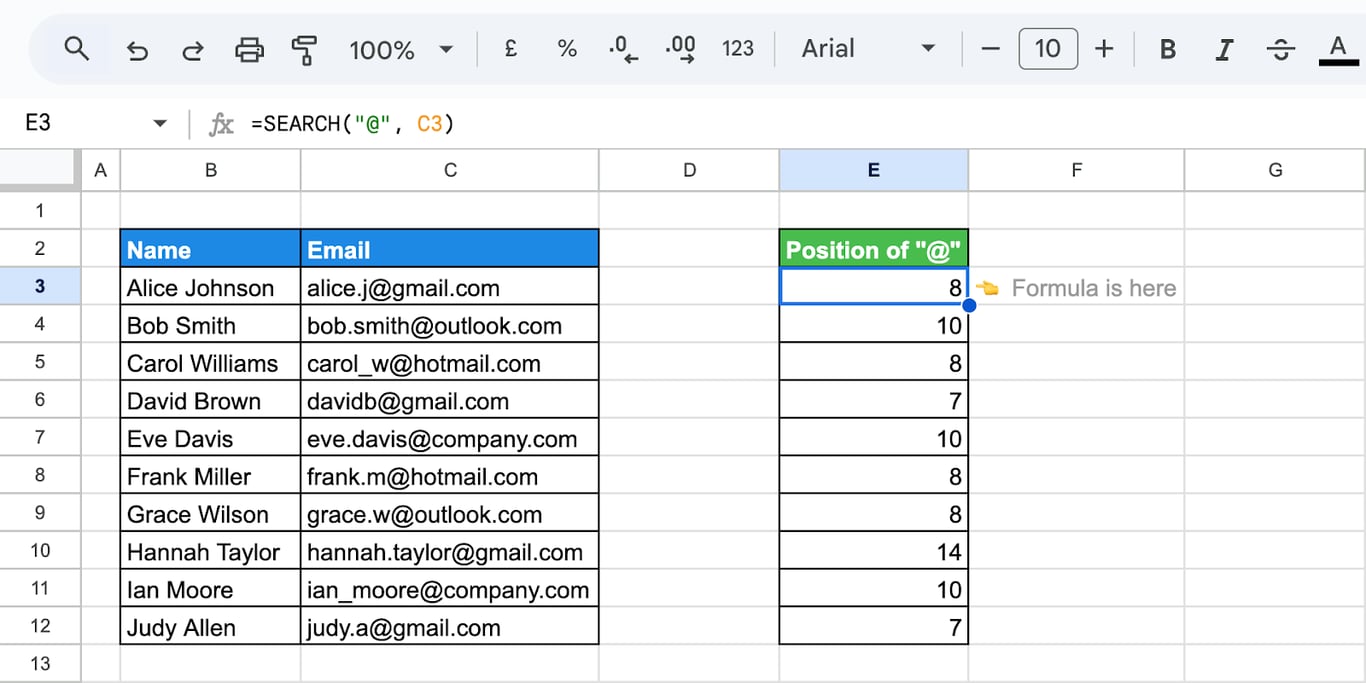
The position tells you where the username ends and the domain begins, which the extraction formulas below build on. The SEARCH function has its own guide with more examples.
Example of FIND
To find the position of the first space in a name:
=FIND(" ", B3)
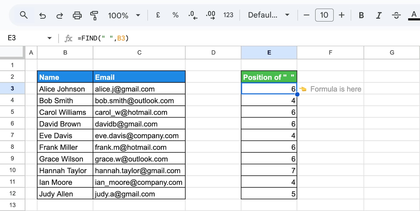
The first space separates the first name from the last name. For a space or an @ sign, case does not matter, and FIND and SEARCH return the same number.
FIND is case-sensitive
FIND matches the exact case. Looking for a lowercase “a”:
=FIND("a", B5)
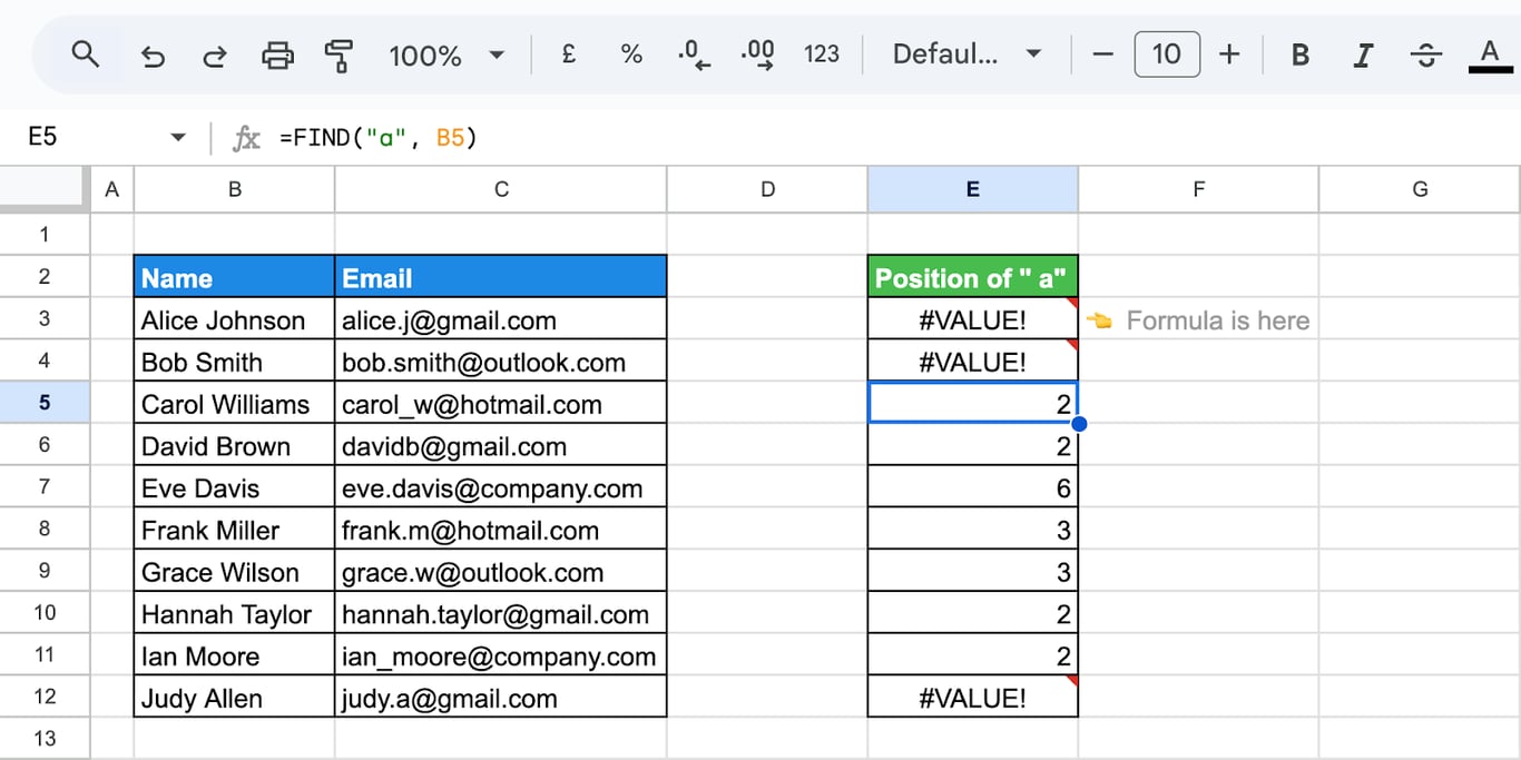
FIND returns the position of the first lowercase “a”. An uppercase “A” does not count, and when the text has no lowercase “a” at all, the result is #VALUE!.
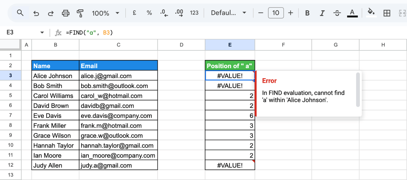
SEARCH would return a position in every case where the letter appears, in either case. Use FIND when the difference matters, for example for codes where “a” and “A” mean different things.
Find a word
Both functions look for any sequence of characters, not just single ones:
=FIND("review", "The product review was positive")
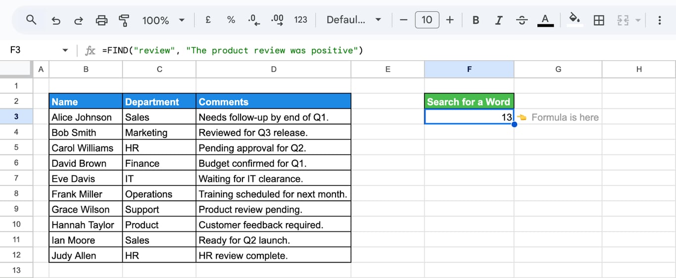
The formula returns 13: the word starts at the thirteenth character.
Start from a later position
The third argument skips the beginning of the text. To look for “a” from the fifth character onward:
=FIND("a", B5, 5)
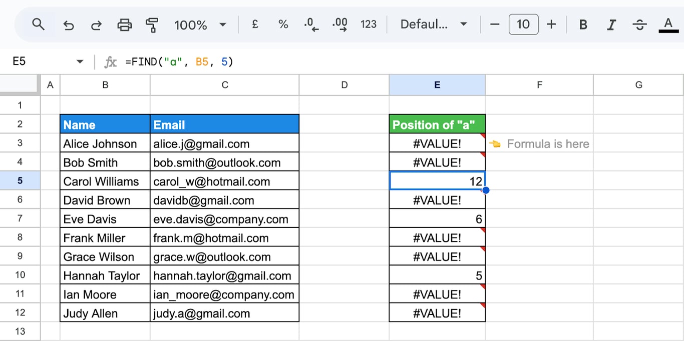
If there is no “a” from that position on, the result is #VALUE!.
Find the second occurrence
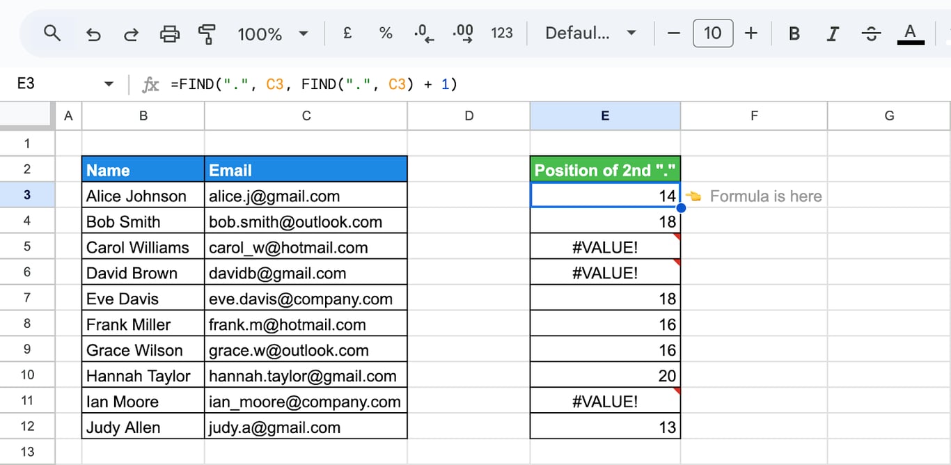
To find the second period in a text, start the search right after the first one:
=FIND(".", C3, FIND(".", C3) + 1)
- FIND(“.”, C3): the position of the first period.
- + 1: the character after it, where the outer FIND starts looking.
OWOX Data Marts
See your first report built in real time. 15 minutes.
- Connect your data warehouse
- Pick your metrics
- Get a live Google Sheets report
In the time it takes to write a ticket. Then imagine never writing that ticket again.
Book a DemoWe'll use your actual use case
SEARCH accepts wildcards
In SEARCH, a question mark stands for any single character and an asterisk for any number of characters. =SEARCH("b?n", "Banana") returns 1, and =SEARCH("n*a", "Banana") returns 3. FIND treats both as ordinary characters: =FIND("b?n", "banana") returns #VALUE!.
Check whether a cell contains text
Check whether a cell contains text
On their own, FIND and SEARCH return a number or an error. To turn that into TRUE and FALSE, wrap them in ISNUMBER: =ISNUMBER(SEARCH("pending", C3)).
A label with IF
=IF(ISERROR(FIND("pending", C3)), "Reviewed", "Needs Attention")
- FIND(“pending”, C3): looks for the lowercase word “pending”.
- ISERROR(…): TRUE when the word is not found.
- IF(…): returns “Reviewed” when it is not found and “Needs Attention” when it is.
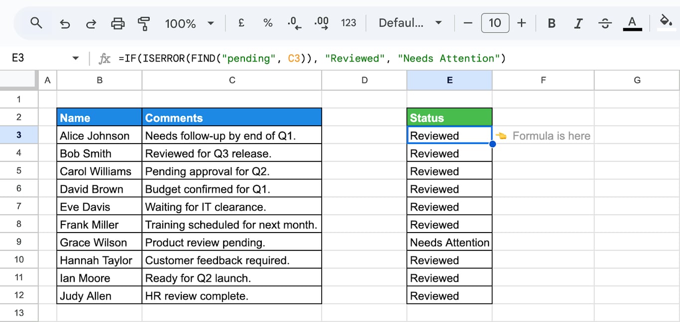
Because FIND is case-sensitive, “Pending” with a capital letter is not matched. Replace FIND with SEARCH to catch both. More on conditions in the guide to the IF function.
A list of matching rows with FILTER
=FILTER(D3:D12, IFERROR(SEARCH("pending", D3:D12), FALSE))
- SEARCH(“pending”, D3:D12): a position for the cells that contain the word, an error for the others.
- IFERROR(…, FALSE): turns the errors into FALSE, so that FILTER can use the result as a condition.
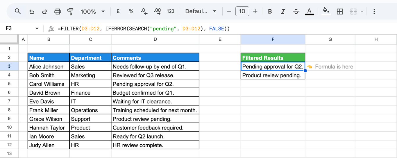
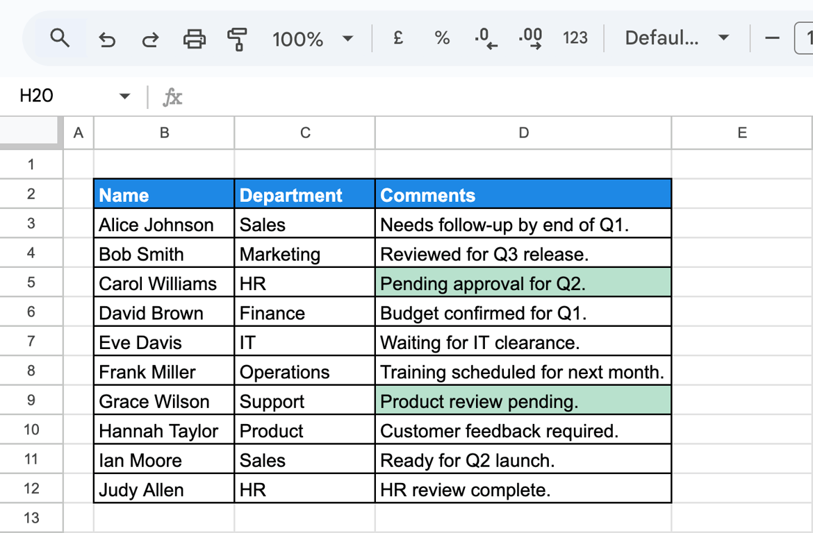
The formula returns the comments that contain “pending”.
Highlighting with conditional formatting
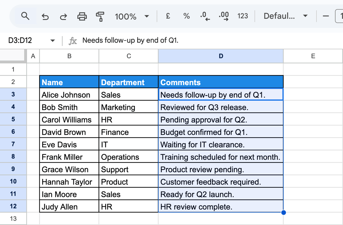
1. Select the range to format.
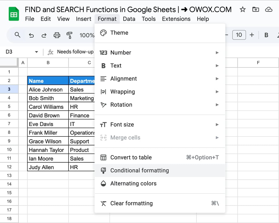
2. Open Format > Conditional formatting.
3. Under Format cells if, choose Custom formula is and enter the formula:
=SEARCH("pending", $D3)
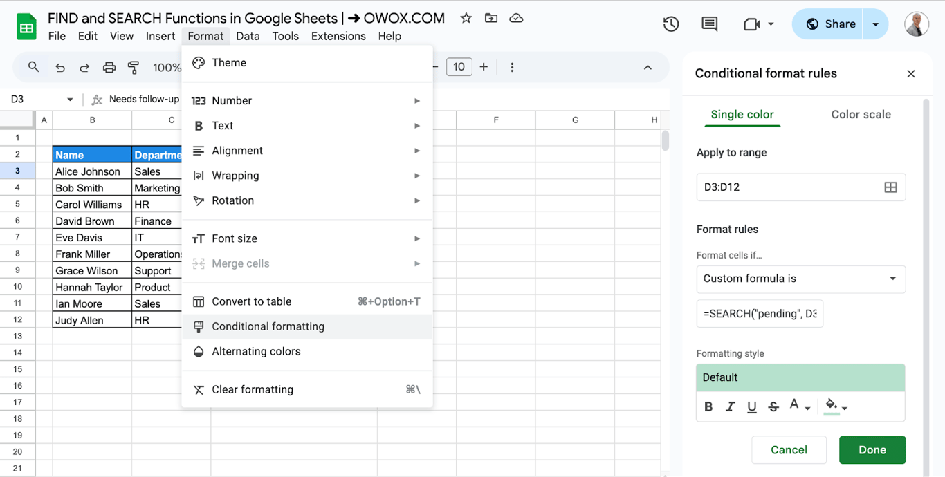
The dollar sign fixes the column, so the whole row is formatted when column D of that row contains the word. The rule in the screenshot is written as =SEARCH("pending", D3:D), which gives the same result here.
Every cell of a range at once
Inside ARRAYFORMULA, one formula returns a position for each cell of a range:
=ARRAYFORMULA(FIND("m", B3:B12))
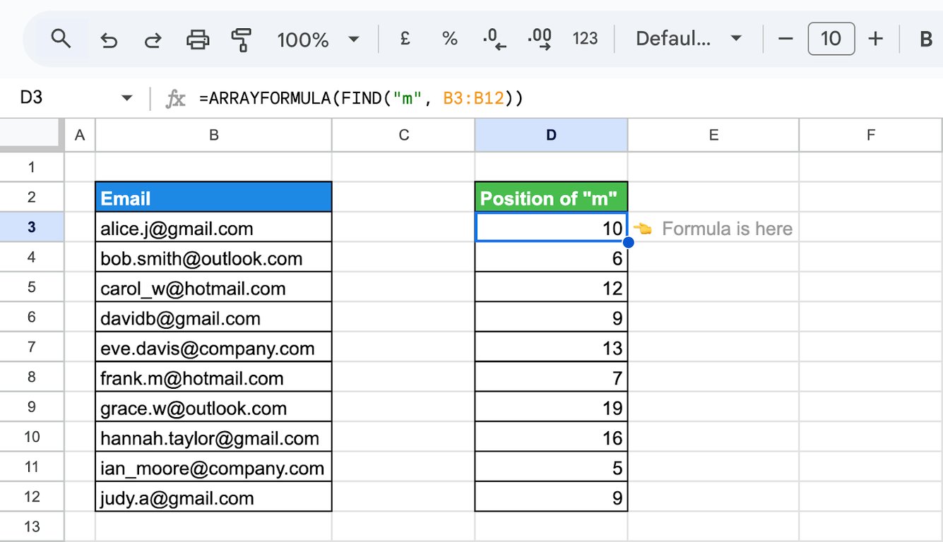
Cells without a lowercase “m” show #VALUE!. Wrap FIND in IFERROR to leave them empty: =ARRAYFORMULA(IFERROR(FIND("m", B3:B12))).
Extract text with FIND and SEARCH
Extract text with FIND and SEARCH
The part before a character
=LEFT(C3, SEARCH("@", C3, 1) - 1)
- SEARCH(“@”, C3, 1): the position of the @ sign.
- - 1: the number of characters before it.
- LEFT(C3, …): that many characters from the start.
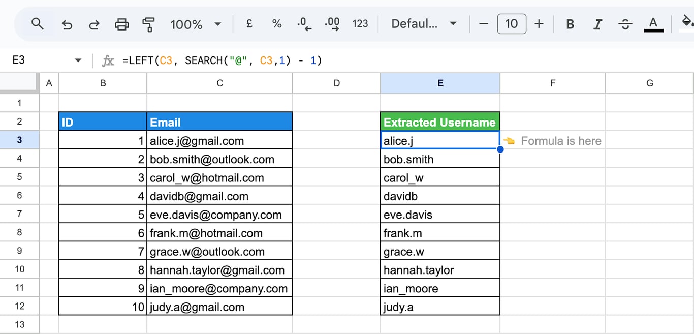
The formula returns the username of each email address.
The part after a character
=RIGHT(C3, LEN(C3) - SEARCH("@", C3))
- LEN(C3): the length of the whole address.
- LEN(C3) - SEARCH(“@”, C3): the number of characters after the @ sign.
- RIGHT(C3, …): that many characters from the end.
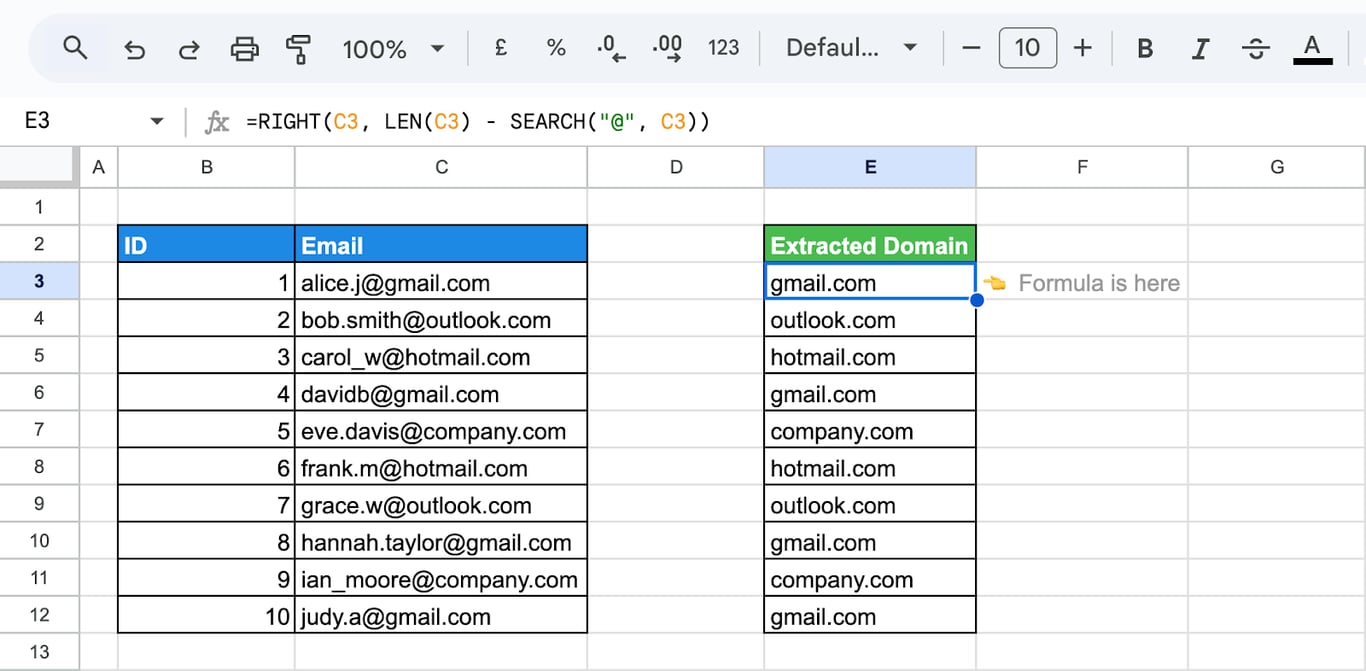
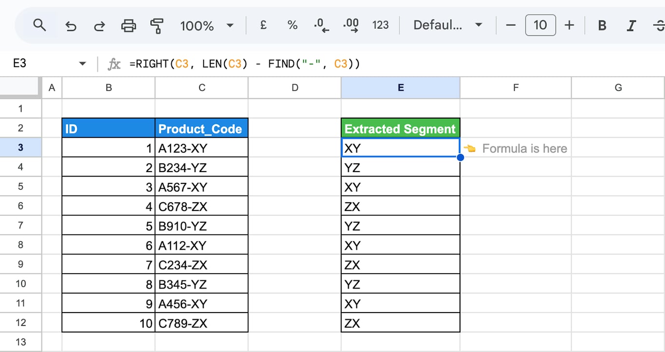
The formula returns the domain. The same pattern with FIND takes the part of a product code after the dash:
=RIGHT(C3, LEN(C3) - FIND("-", C3))
The first word
=MID(C3, 1, FIND(" ", C3) - 1)
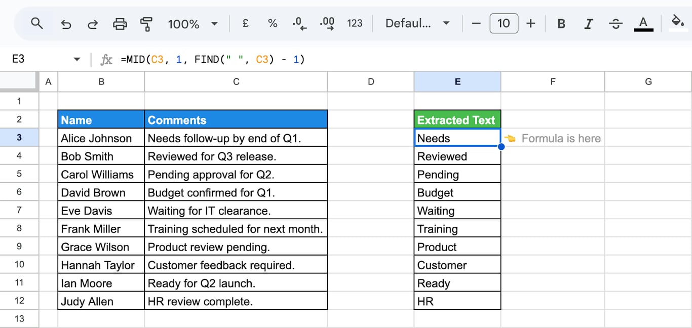
FIND returns the position of the first space, and MID takes the characters before it. =LEFT(C3, FIND(" ", C3) - 1) does the same. The guide to LEFT, RIGHT and MID covers these functions.
Build a text from the extracted part
=CONCATENATE("Hello, ", LEFT(B3, FIND("@", B3) - 1), "! Welcome to our service.")
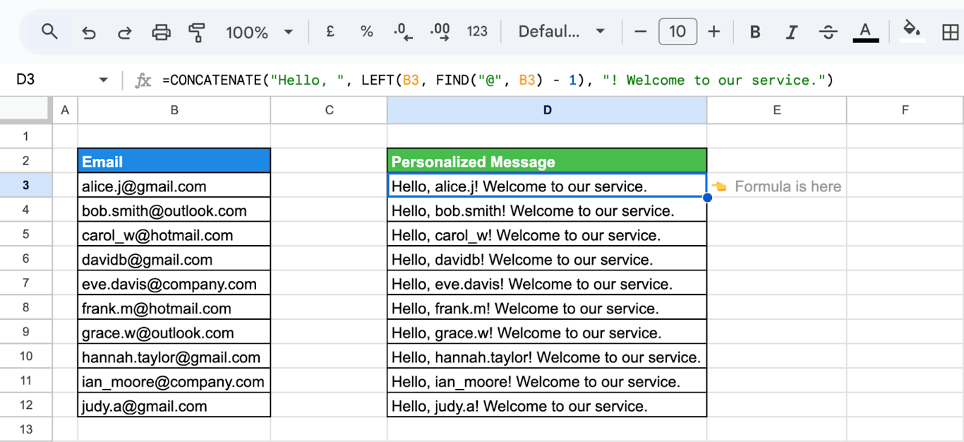
The middle part is the username taken from the email address; CONCATENATE puts the fixed text around it.
Replace text at a found position
Replace text at a found position
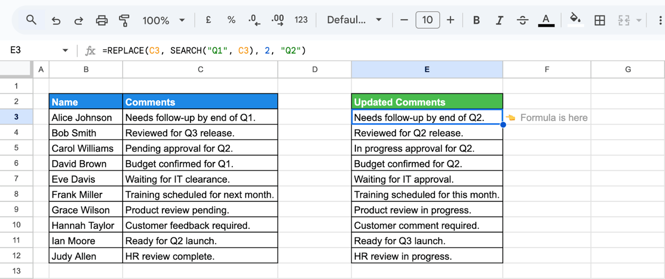
REPLACE needs a position and a length, and SEARCH supplies the position. To change “Q1” to “Q2”:
=REPLACE(C3, SEARCH("Q1", C3), 2, "Q2")
- SEARCH(“Q1”, C3): where “Q1” starts.
- 2: the number of characters to replace.
- “Q2”: the new text.
Do not pass the result of FIND to SUBSTITUTE as its fourth argument. That argument is the number of the occurrence to replace, not a position: =SUBSTITUTE("banana", "a", "@", FIND("a", "banana")) returns ban@na, because FIND returns 2 and SUBSTITUTE then replaces the second “a”. To replace the first occurrence, use =SUBSTITUTE(B3, "a", "@", 1).
Errors in FIND and SEARCH
⚠️ Error: #VALUE!
✅ Solution: This is the only error the two functions return for the data, and it has three causes. The text was not found. With FIND, the text is there but in a different case. Or the starting position is 0, negative, or beyond the end of the text. To show something else instead, use IFERROR: =IFERROR(FIND("x", B3), 0).
⚠️ Error: #NAME?
✅ Solution: The function name is misspelled, or the text to look for is not in quotes.
⚠️ Error: #ERROR! (formula parse error)
✅ Solution: A quote or a parenthesis is missing.
⚠️ Error: A position is returned, but the wrong one.
✅ Solution: Both functions return the first match. If the text appears more than once, use the starting position to move past the earlier ones.
Related Google Sheets functions
Related Google Sheets functions
Functions that are often used next to FIND and SEARCH, each with its own guide:
- SEARCH: The case-insensitive search in detail.
- REGEX functions: Match, extract and replace text by pattern.
- SUBSTITUTE: Replaces one text with another, everywhere or at a given occurrence.
- LEFT/RIGHT/MID: Extracts a set number of characters from the start, end or middle of a text string.
- SPLIT: Cuts a text into columns at a delimiter.
- MATCH: Returns the position of a value in a range of cells, where FIND returns a position inside one cell.
- CHAR: Returns the character for a Unicode number, useful for symbols and line breaks.
- Wrap text: Keeps long text visible inside a cell by breaking it onto several lines.
Text formulas repair what the export broke
Text formulas repair what the export broke
Most formulas in this guide take apart a value that was one field in the system it came from: a domain inside an email address, a region inside a campaign name, a status inside a comment. In the source those are often separate columns. They become one string on the way into the spreadsheet, and FIND and SEARCH are then used to cut it apart again.
The OWOX Data Marts extension for Google Sheets covers that half. A data analyst publishes a data mart (a table or an SQL query in your data warehouse) and makes it available for reports. In Sheets you open the extension, pick the data mart, tick the columns you want and run it. The rows land in a tab, ready for your formulas.
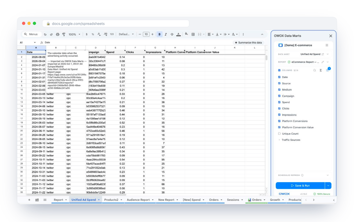
What changes for the person who maintains the sheet:
- Refresh replaces re-export. Refresh current report in the extension menu re-runs the same pull, and a scheduled refresh keeps the tab current without anyone touching it.
- The source is written on the sheet. The header cell of an imported tab carries a note with the data mart it came from, the time of the import and a link to the report.
- No SQL and no warehouse access needed. The analyst decides which data marts and columns are available. You choose from that list.
The extension does not write or change the analyst’s SQL. When the analyst exposes the parts as columns, the sheet receives them ready to use, and the text functions are left for the cases that really are free text. The extension comes with the OWOX Cloud plans of OWOX Data Marts; spreadsheet reporting describes both ways data reaches a sheet.
Turn your data into decisions.
Governed data marts give you the clean foundation ML needs to actually work.
- No AI hallucinations
- Analyst-governed definitions
- Every number traces to SQL
Frequently Asked Questions
How do I handle errors when using FIND or SEARCH in Google Sheets?
Both functions return #VALUE! when the text is not found. Wrap them in IFERROR to return something else: =IFERROR(FIND("text", A2), "Not found"). To get TRUE or FALSE, use =ISNUMBER(SEARCH("text", A2)).
Can I combine FIND or SEARCH with other formulas in Google Sheets?
Yes. =IF(ISNUMBER(SEARCH("text", A2)), "Found", "Not found") returns a label, =LEFT(A2, FIND("@", A2) - 1) extracts the part before a character, and =FILTER(A2:A, ISNUMBER(SEARCH("text", A2:A))) lists the rows that contain the text.
Can I use FIND or SEARCH across multiple sheets in Google Sheets?
FIND and SEARCH look inside one cell, so they do not search a sheet. To check a range on another tab, add the tab name: =ARRAYFORMULA(IFERROR(SEARCH("text", Sheet2!A2:A20))). To look for a value across the whole file by hand, press Ctrl + F and choose to search all sheets in the find and replace dialog.
How can I perform a case-insensitive search in Google Sheets?
Use SEARCH: =SEARCH("text", A2) finds the text whatever its case and returns its position. SEARCH also accepts the wildcards ? and *. FIND, by contrast, matches the exact case.
How do I use the FIND function to locate specific text in Google Sheets?
Type =FIND("text", A2), with the text to look for in quotes and the cell to look in as the second argument. The function returns the position of the first match, counted in characters from the left, and #VALUE! when the text is not there. FIND is case-sensitive.
What is the difference between the FIND and SEARCH functions in Google Sheets?
The FIND function in Google Sheets is case-sensitive and does not support wildcard characters, while the SEARCH function is case-insensitive and allows the use of wildcards (* and ?). Both functions return the position of a substring within a text, but suit different needs based on sensitivity and flexibility.