Day of the week and week number in Google Sheets: WEEKDAY, WEEKNUM and ISOWEEKNUM
WEEKDAY returns the day of the week of a date as a number, TEXT returns it as a name, and WEEKNUM and ISOWEEKNUM return the week of the year. This guide covers the type argument of each, worked examples, combinations with IF, COUNTIF, INDEX and VLOOKUP, and the errors you can meet.

To get the day of the week from a date in Google Sheets, use =WEEKDAY(A1). It returns a number from 1 (Sunday) to 7 (Saturday). For the name of the day instead of a number, use =TEXT(A1, “dddd”), which returns “Monday”, “Tuesday” and so on. For the week of the year, use =WEEKNUM(A1), or =ISOWEEKNUM(A1) for ISO weeks.
| You want | Formula | Result for a Wednesday |
|---|---|---|
| Day of the week as a number, week starting Sunday | =WEEKDAY(A1) |
4 |
| Day of the week as a number, week starting Monday | =WEEKDAY(A1, 2) |
3 |
| Name of the day | =TEXT(A1, "dddd") |
Wednesday |
| Short name of the day | =TEXT(A1, "ddd") |
Wed |
| Week of the year | =WEEKNUM(A1) |
1 to 53 |
| ISO week of the year | =ISOWEEKNUM(A1) |
1 to 53 |
The rest of this guide explains the three functions and their type arguments, then shows them in formulas with conditional formatting, IF, COUNTIF, INDEX and MATCH, VLOOKUP and DATE.
WEEKDAY, WEEKNUM and ISOWEEKNUM: syntax and examples
WEEKDAY, WEEKNUM and ISOWEEKNUM: syntax and examples
WEEKDAY
WEEKDAY returns a number representing the day of the week of a date. By default 1 is Sunday, 2 is Monday and so on up to 7 for Saturday.
Syntax of WEEKDAY
The syntax of the WEEKDAY function in Google Sheets is:
=WEEKDAY(date, [type])
Let’s break it down:
- date: The date for which you want to find the day of the week. This can be a date entered directly, a cell reference, or a formula that returns a date.
- type (optional): Specifies the numbering system for days of the week.
Google Sheets accepts three types:
- 1 (default): Numbers the days from Sunday = 1 to Saturday = 7.
- 2: Numbers the days from Monday = 1 to Sunday = 7.
- 3: Numbers the days from Monday = 0 to Sunday = 6.
Example of WEEKDAY
To find the day of the week of each employee’s birthday in column C:
=WEEKDAY(C3, 1)
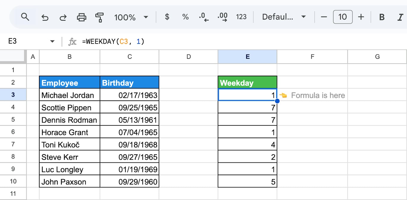
With type 1, the result counts from Sunday = 1 to Saturday = 7. The number is what you need for calculations and conditions. For a label a person will read, =TEXT(C3, "dddd") returns the name of the day directly.
WEEKNUM
WEEKNUM returns the week of the year a date falls in, as a number from 1 to 53. Week 1 is the week that contains January 1.
Syntax of WEEKNUM
The syntax of the WEEKNUM function is as follows:
=WEEKNUM(date, [type])
Let’s explain:
- date: The date for which you want to find the week number.
- type (optional): Specifies the day on which the week starts.
The type values:
- 1 (default): the week starts on Sunday.
- 2: the week starts on Monday.
- 11 to 17: the week starts on Monday (11), Tuesday (12), Wednesday (13), Thursday (14), Friday (15), Saturday (16) or Sunday (17).
- 21: ISO 8601 numbering: the week starts on Monday, and week 1 is the week that contains the first Thursday of the year. This is the same result as ISOWEEKNUM.
With every type except 21, January 1 is always in week 1, so the first week of a year can be shorter than seven days.
Example of WEEKNUM
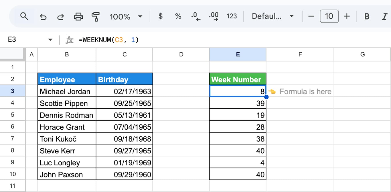
To find the week of the year of each employee’s birthday:
=WEEKNUM(C3, 1)
With type 1, weeks begin on Sunday.
ISOWEEKNUM
ISOWEEKNUM returns the ISO 8601 week number of a date. In this system every week starts on Monday and has seven days, and week 1 is the week that contains the first Thursday of the year. As a consequence, January 1 can belong to the last week of the previous year, and December 31 to week 1 of the next.
ISO weeks are the standard in most of Europe and in international reporting. =WEEKNUM(date, 21) returns the same number; pick one of the two and use it throughout a sheet.
Syntax of ISOWEEKNUM
=ISOWEEKNUM(date)
- date: The date to evaluate: a cell with a date, or a formula that returns one.
Example of ISOWEEKNUM
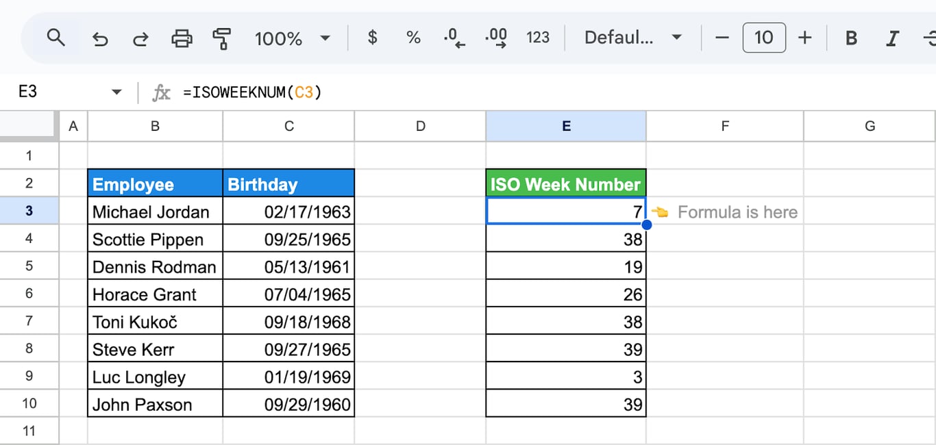
To find the ISO week of each employee’s birthday:
=ISOWEEKNUM(C3)
For a birthday on 02/17/1963, the function returns 7: the date falls in the seventh ISO week of that year.
Basic examples of WEEKDAY and WEEKNUM
Basic examples of WEEKDAY and WEEKNUM
Using WEEKDAY to identify the day of the week
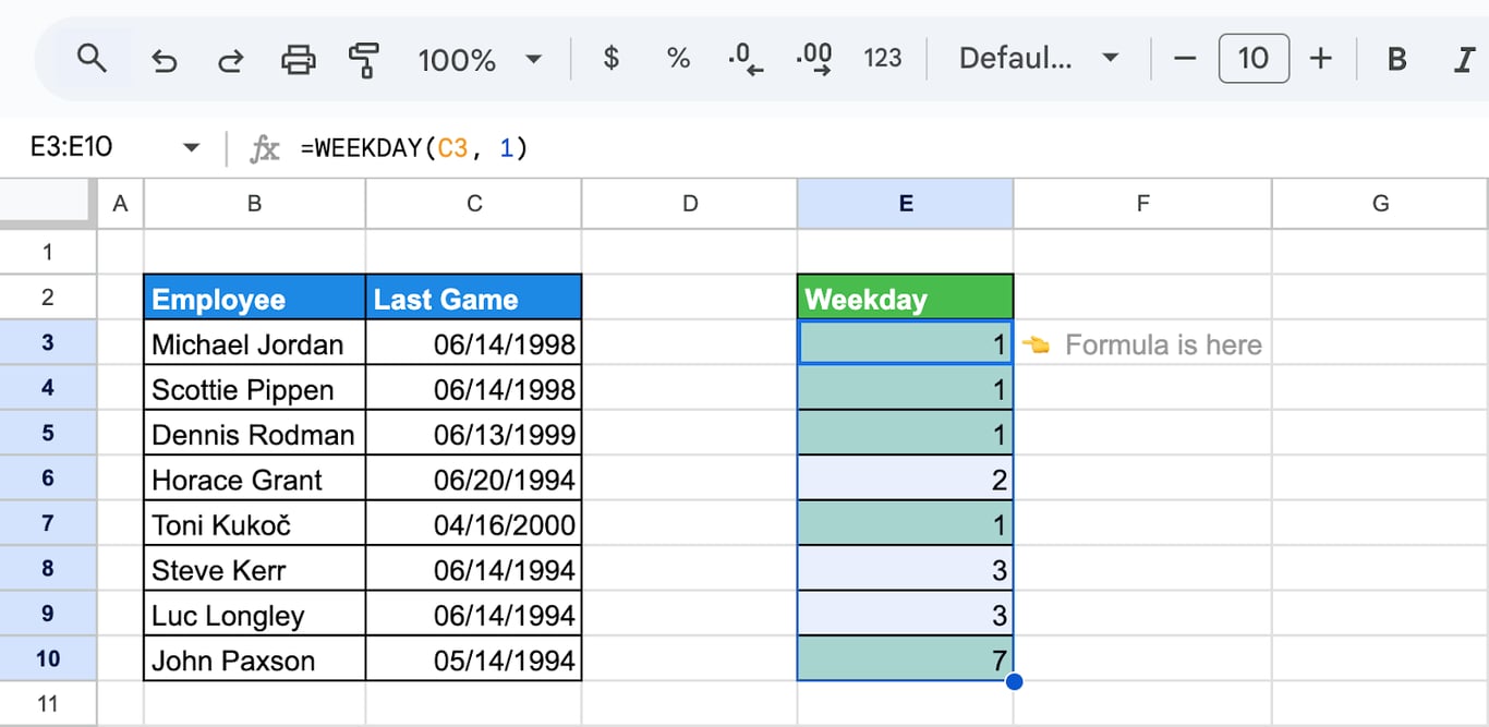
The examples use a table of Chicago Bulls players with the date of each player’s last game in column C. To find the day of the week of the last game:
=WEEKDAY(C3, 1)
Here’s the breakdown:
- C3: The last game day.
- 1: Numbers the days from Sunday = 1 to Saturday = 7, where 1 represents Sunday and 7 represents Saturday.
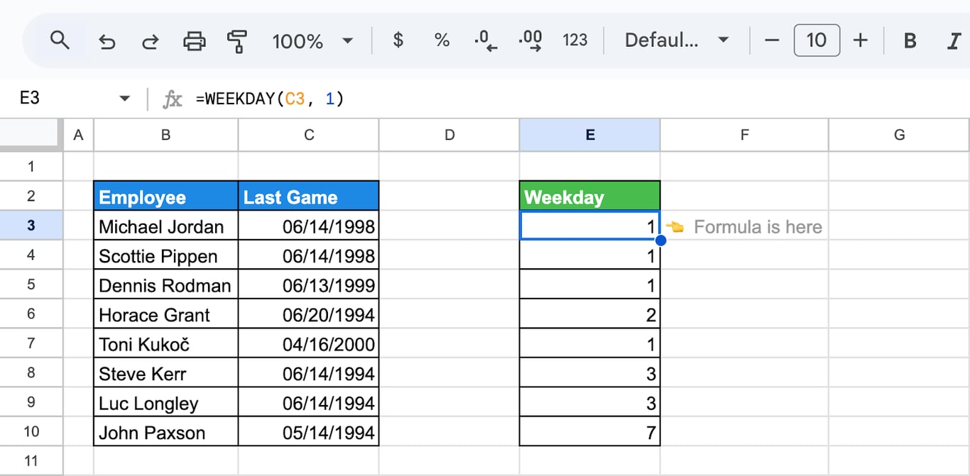
Copy the formula down to get the weekday of every game.
Customizing the WEEKDAY function with the type argument
In much of the world the week starts on Monday. Set the type to 2 and WEEKDAY counts from Monday = 1 to Sunday = 7:
=WEEKDAY(C3, 2)
Breakdown of the formula:
- C3: The last game day.
- 2: Numbers the days from Monday = 1 to Sunday = 7.
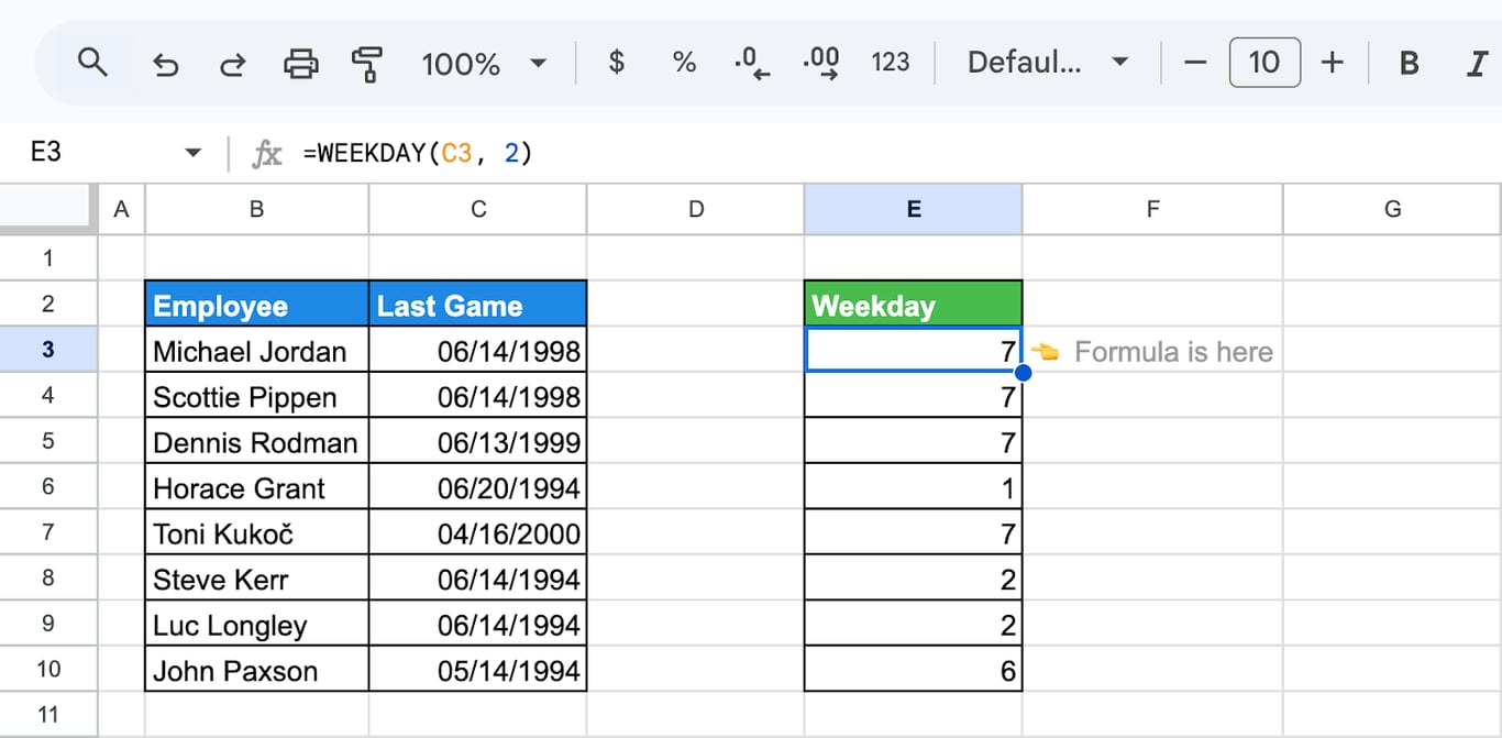
Type 2 also makes weekend tests simple: Saturday and Sunday are the only results greater than 5.
Adding the word “Week” to the WEEKNUM function
A bare number in a report is easy to misread. Join the text “Week “ to the result with the & operator:
="Week " & WEEKNUM(C3)
For a date in cell C3 such as 02/17/1963, the result is “Week 7”.
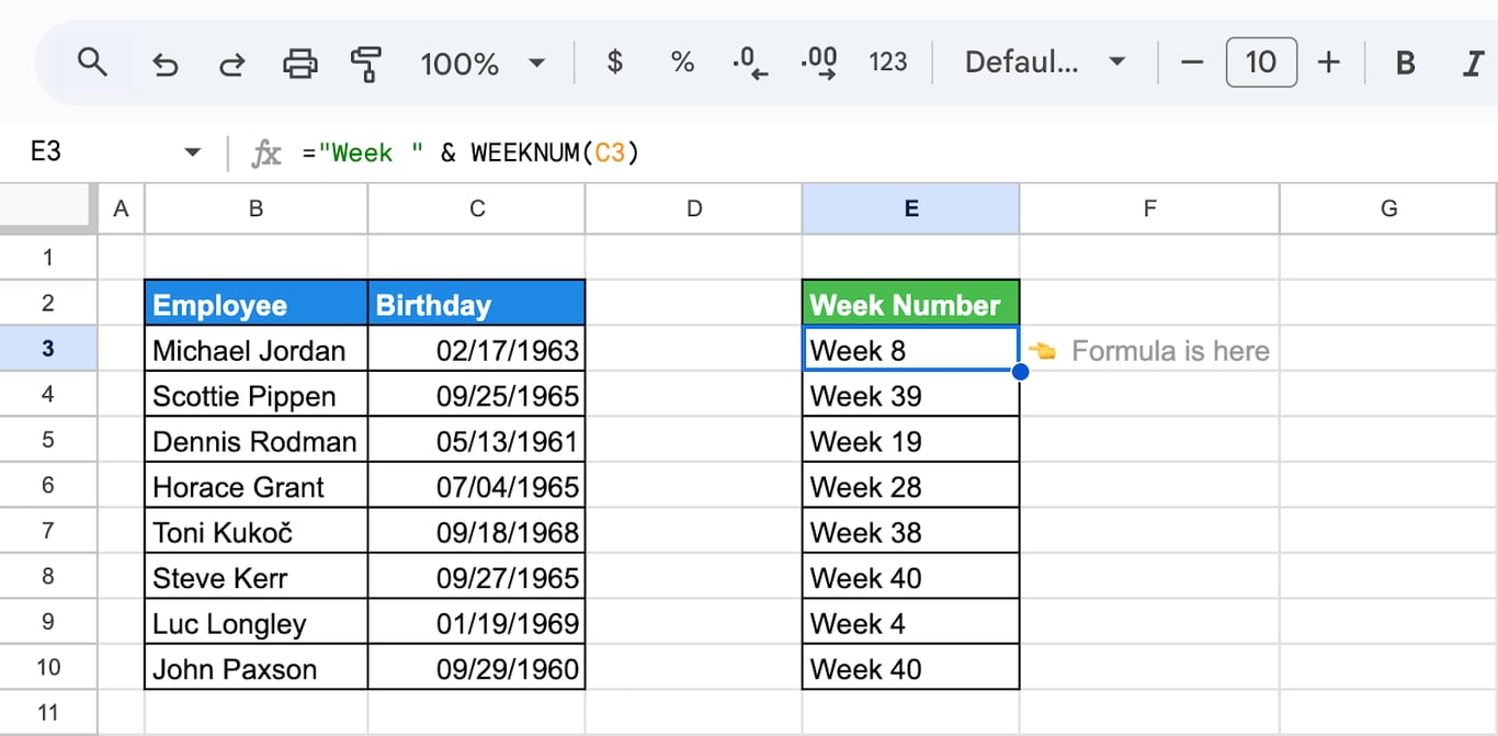
The result is text, so it can no longer be used in calculations. Keep the plain WEEKNUM in a helper column if you need to sort or compare by week.
Calculate the number of weeks in between two dates using WEEKNUM
Subtracting two week numbers gives the number of calendar weeks between two dates in the same year:
=WEEKNUM(D3) - WEEKNUM(C3)
WEEKNUM(D3) is the week of the later date and WEEKNUM(C3) the week of the earlier one.
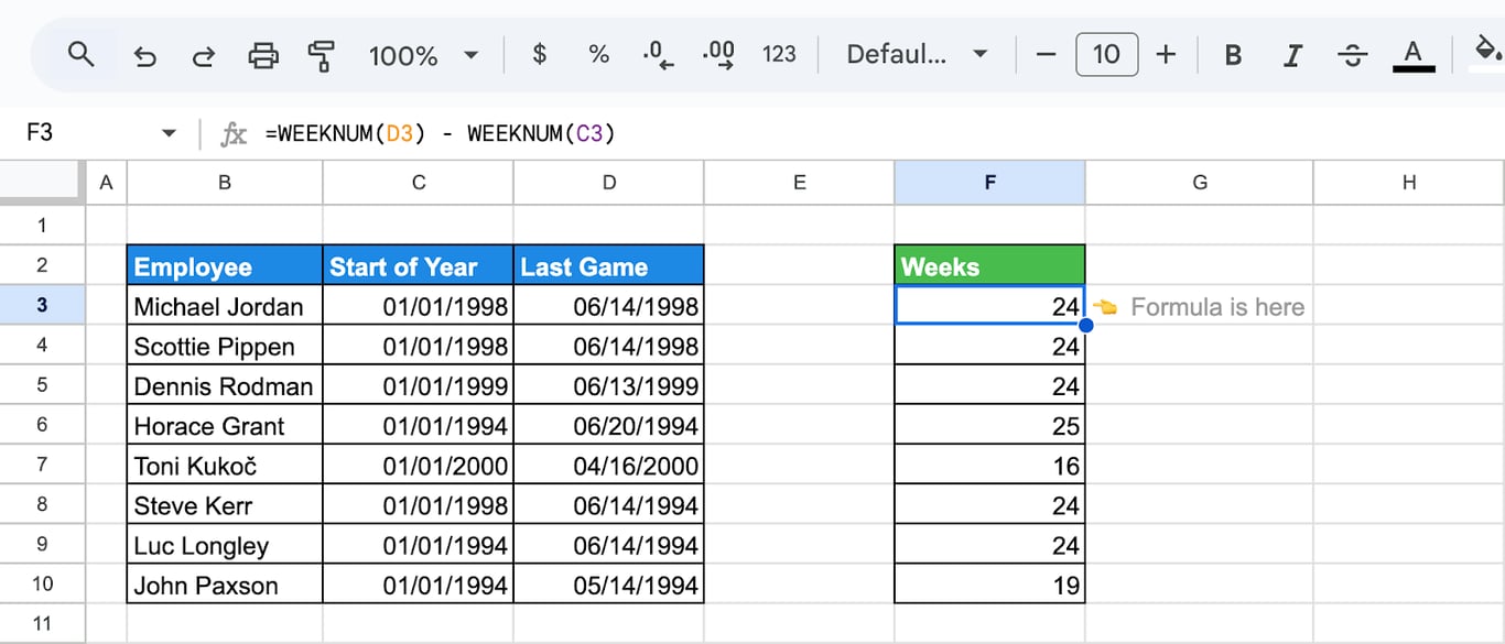
This is an approximation, and it breaks when the two dates are in different years, because week numbers start again at 1. For the number of full weeks between any two dates, divide the day difference by seven:
=INT((D3 - C3) / 7)
Organizing team events by ISO week numbers in Google Sheets
Each player has a contract renewal date in column D. To plan the renewals by ISO week:
=ISOWEEKNUM(D3)
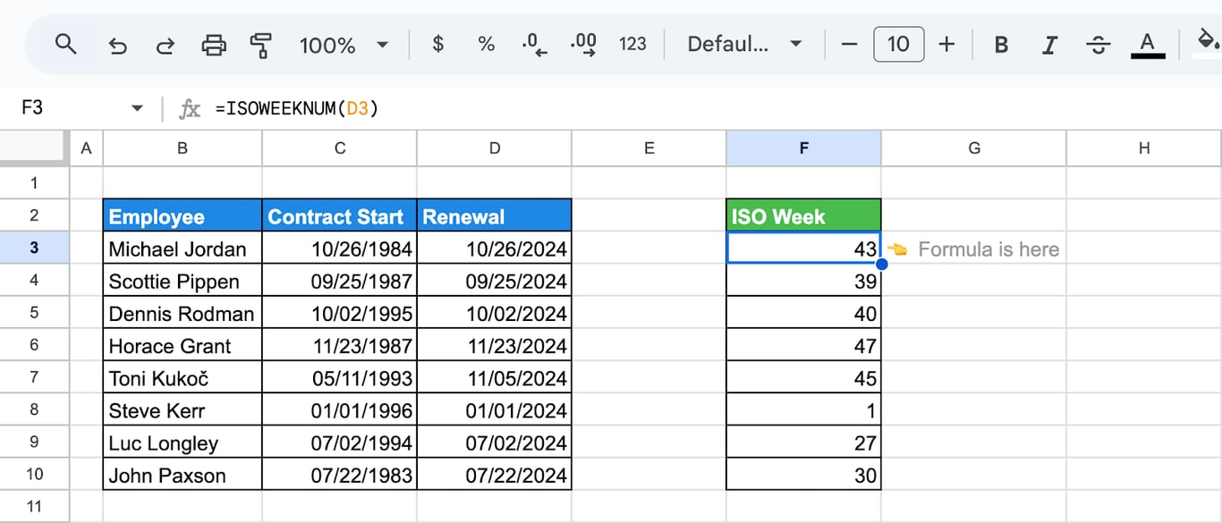
Sort or filter by the result to see which renewals fall in the same week.
OWOX Data Marts
See your first report built in real time. 15 minutes.
- Connect your data warehouse
- Pick your metrics
- Get a live Google Sheets report
In the time it takes to write a ticket. Then imagine never writing that ticket again.
Book a DemoWe'll use your actual use case
WEEKDAY and WEEKNUM in practice
WEEKDAY and WEEKNUM in practice
Highlighting weekends with conditional formatting and WEEKDAY
A custom formula in conditional formatting can color every date that falls on a weekend. To highlight the last games played on a Saturday or Sunday:
- Select the range you want to apply formatting to (e.g., C3:C11 for the “Last Game” dates).
- Go to Format → Conditional formatting.
- Under Format cells if, choose Custom formula is and enter:
=OR(WEEKDAY(C3)=1, WEEKDAY(C3)=7)
The formula is true when the day is Sunday (1) or Saturday (7). Write it for the first cell of the range; Google Sheets applies it to the rest.
- Choose a fill color and click Done.
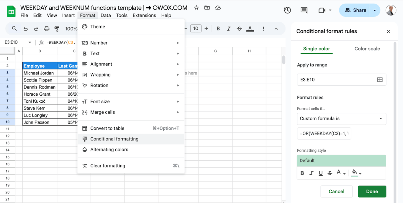
The weekend dates are now filled with the chosen color:
Comparing different types of week counting using WEEKNUM
The same date can fall in different weeks depending on the type. This table applies types 1, 2, 14 and 21 to the same dates. The last column uses:
=WEEKNUM(C3, 21)
Let’s explain:
- C3: The date to evaluate.
- 21: ISO 8601 numbering: weeks start on Monday, and week 1 is the week that contains the first Thursday of the year.
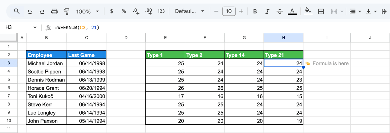
The numbers differ most around the turn of the year and for dates near the start or end of a week. Before two people compare “week 14”, they need to agree on the type.
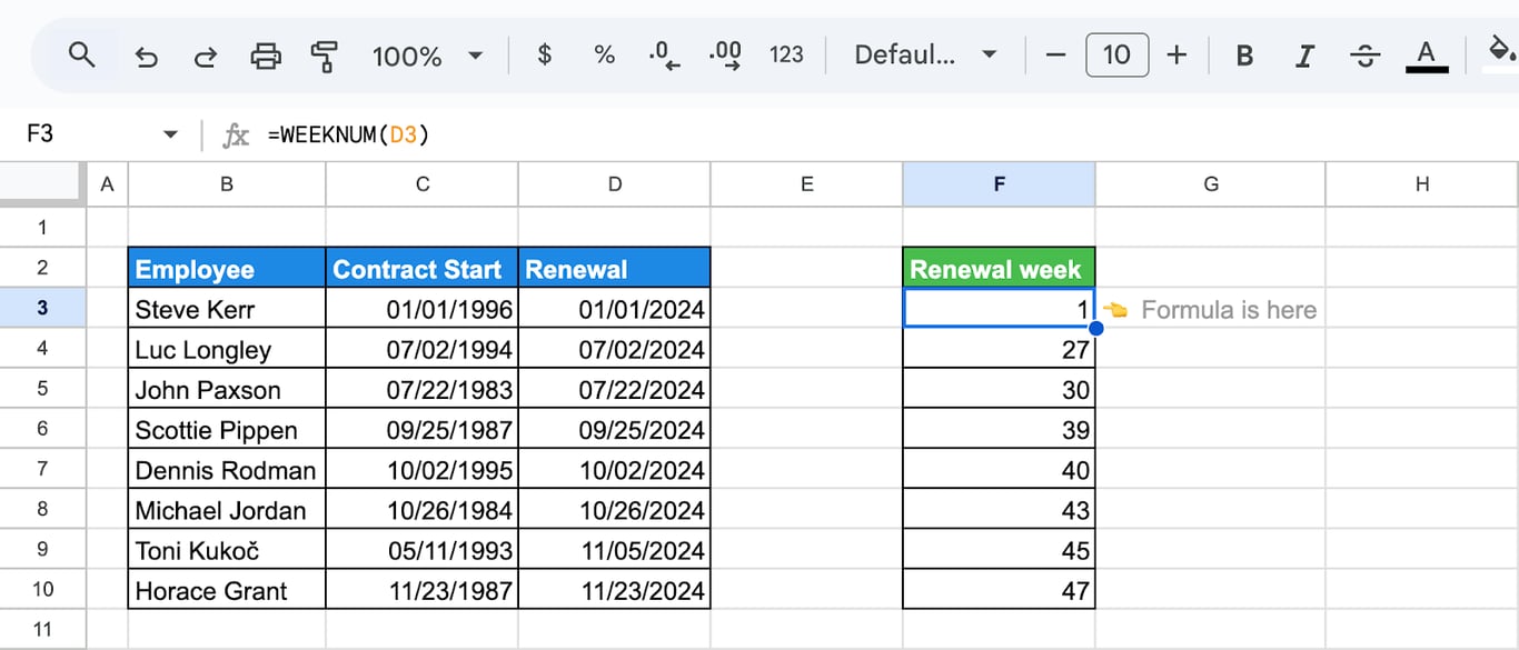
Categorizing project tasks by week using WEEKNUM
To group the contract renewals by week of the year:
=WEEKNUM(D3)
Sort the sheet by the week column and the renewals line up in the order the paperwork has to be prepared.
Analyzing results by ISO week
A week column turns daily records into a weekly series. The table lists the Chicago Bulls games of November 1995 with the date in column C and the score next to it. Add the ISO week of each game:
=ISOWEEKNUM(C3)
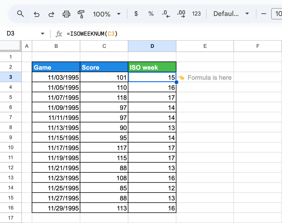
To analyze the total scores by week, we’ll create a pivot table:
- Select the data range B2:D16
- Go to Data > Pivot Table to set up a new pivot table.
In the pivot table:
- Add ISO Week to Rows.
- Add Score to Values, setting the aggregation to SUM.
Visualize weekly score trends:
- Select the pivot table.
- Insert a chart with Insert → Chart. A line chart suits a series over time.
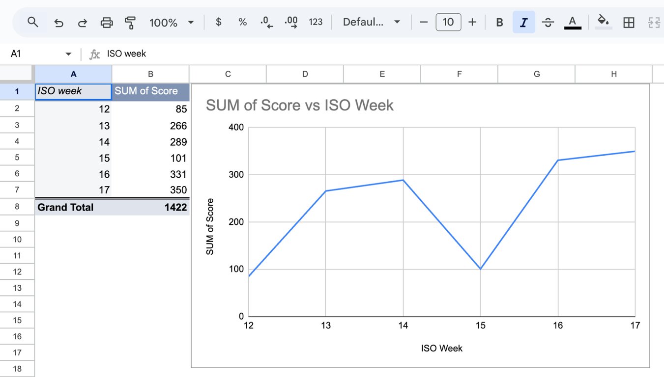
For data that spans more than one year, group by year and week together, or week 5 of two different years will be added up as one.
Combining WEEKDAY and WEEKNUM with other functions
Combining WEEKDAY and WEEKNUM with other functions
Displaying weekday names using WEEKDAY and CHOOSE functions
CHOOSE picks the item at a given position from a list. Feed it the WEEKDAY number and it returns the name of the day:
=CHOOSE(WEEKDAY(C3,1),"Sunday","Monday","Tuesday","Wednesday","Thursday","Friday","Saturday")
Here’s how it works:
- WEEKDAY: extracts the numeric day of the week from the date in column C (e.g., 1 for Sunday, 7 for Saturday).
- CHOOSE: maps these numbers to their respective weekday names using a predefined list: “Sunday”, “Monday”, “Tuesday”, ….
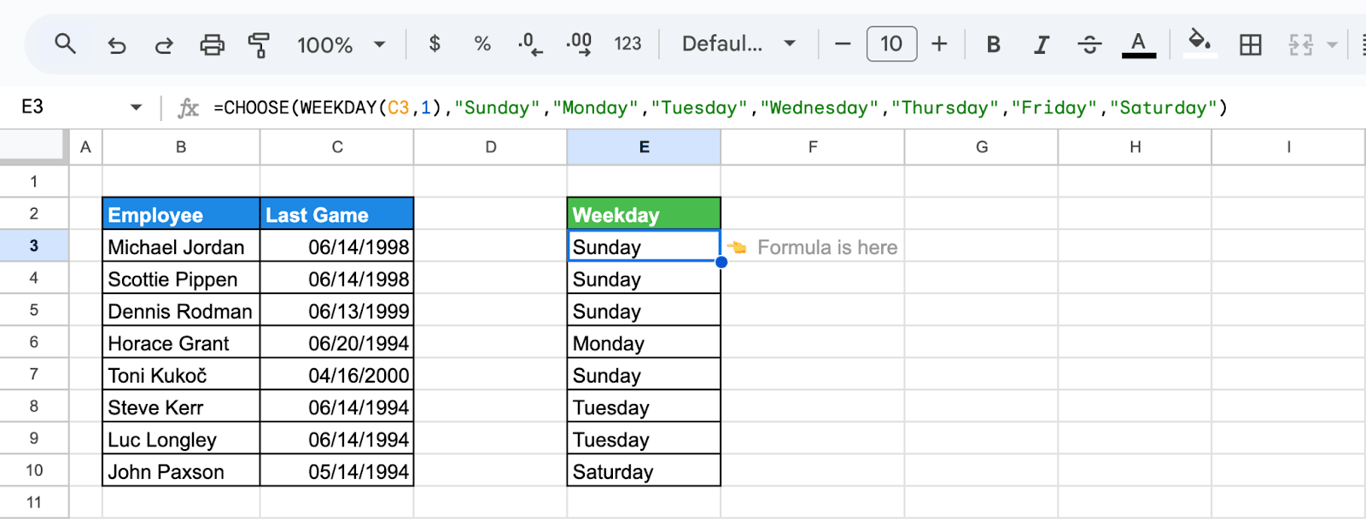
For standard day names, =TEXT(C3, "dddd") is shorter and follows the language of the spreadsheet. CHOOSE is the right tool when the labels are your own, for example “Office”, “Remote” or “Closed” for each day of the week.
WEEKDAY function with COUNTIF and ARRAYFORMULA
With ARRAYFORMULA, WEEKDAY works on a whole range, and COUNTIF counts how often a given day appears.

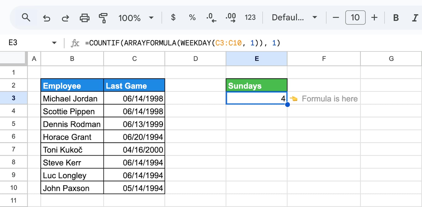
To count how many of the last games were played on a Sunday:
=COUNTIF(ARRAYFORMULA(WEEKDAY(C3:C10, 1)), 1)
Here’s the breakdown:
- WEEKDAY(C3:C10,1): Converts each date in the range C3:C10 into a numeric representation of the weekday (e.g., Monday = 2, Sunday = 1).
- ARRAYFORMULA: ensures the WEEKDAY function is applied to the entire range.
- COUNTIF: Counts how many of these numeric weekday results are equal to 1 (Sunday).
The formula calculates that 4 games occurred on a Sunday. You can adapt this method to count other days of the week by simply replacing 1 (Sunday) in the formula with another number corresponding to the desired weekday (e.g., 2 for Monday, 3 for Tuesday, etc.).
WEEKDAY with IF function
With the IF function, WEEKDAY sorts dates into groups.

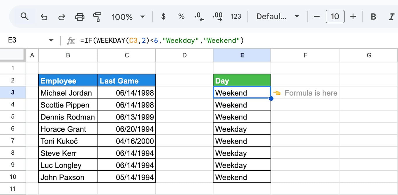
To label each last game as a weekday or a weekend game:
=IF(WEEKDAY(C3,2)<6,"Weekday","Weekend")
Let’s explain:
- WEEKDAY(C3,2): returns a number (1 for Monday, 7 for Sunday) based on the date in C3.
- IF: checks if the number is less than 6 (Monday to Friday). If true, it outputs “Weekday”, otherwise “Weekend”.
WEEKDAY with INDEX and MATCH function
With INDEX and MATCH, you can find the row whose date falls on a given day.

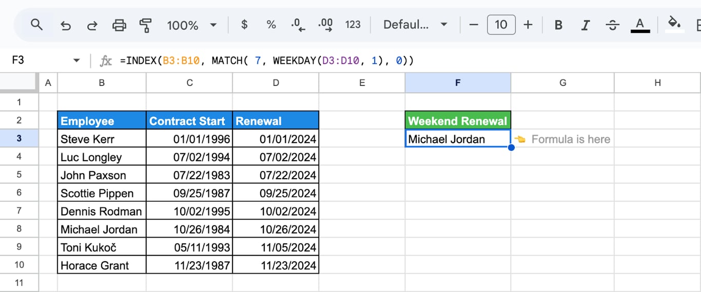
To find the player whose contract renewal falls on a Saturday:
=INDEX(B3:B10,MATCH(7,WEEKDAY(D3:D10,1),0))
Let’s explain:
- WEEKDAY(D3:D10, 1): calculates the weekday for each date in the Renewal column (1 = Sunday, 7 = Saturday).
- MATCH(7, WEEKDAY(D3:D10, 1), 0): finds the first instance of Saturday (7 in the WEEKDAY system).
- INDEX(B3:B10, …): retrieves the corresponding player name from the Employee column.
The formula returns Michael Jordan, the first player in the list with a Saturday renewal. A renewal date on a day the office is closed is worth knowing about in advance.
MATCH returns the first match only. To list every row that falls on a Saturday, use =FILTER(B3:B10, WEEKDAY(D3:D10, 1) = 7).
WEEKDAY with VLOOKUP and TODAY function
WEEKDAY(TODAY()) returns the number of the current day, and VLOOKUP can use it to fetch whatever belongs to today from a table.

Suppose the team wears a different uniform color on each day of the week. A reference table lists the weekday number, the day name and the color. To show today’s color:
=VLOOKUP(WEEKDAY(TODAY(), 2), B3:D9, 3, FALSE)
Breakdown:
- TODAY(): retrieves the current date.
- WEEKDAY(): converts this date into a weekday number (1 = Monday, 7 = Sunday) using the type 2 argument.
- VLOOKUP: searches for the weekday number and retrieves the corresponding uniform color.
- FALSE: ensures an exact match is required.
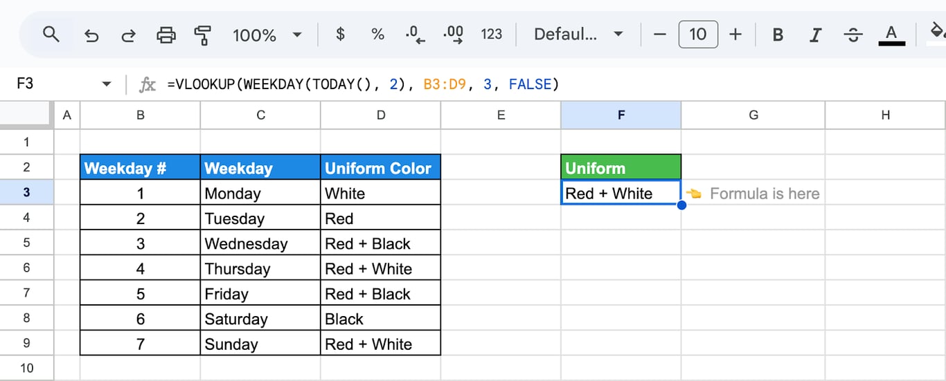
The result changes by itself every day.
Dynamic date calculations using WEEKNUM with the DATE function
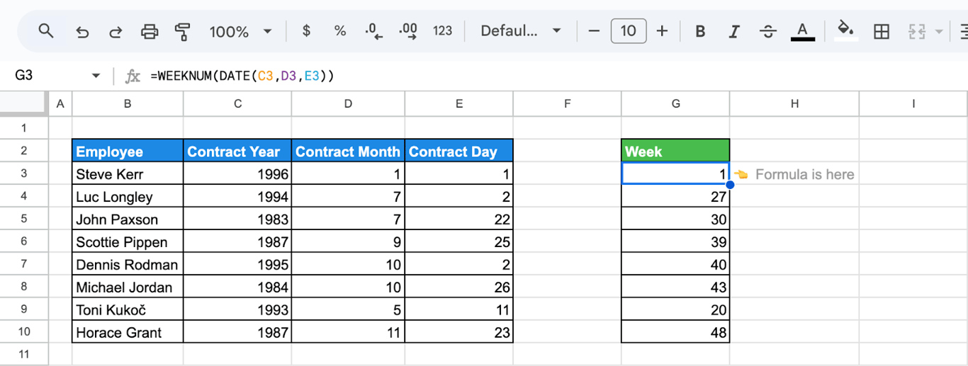
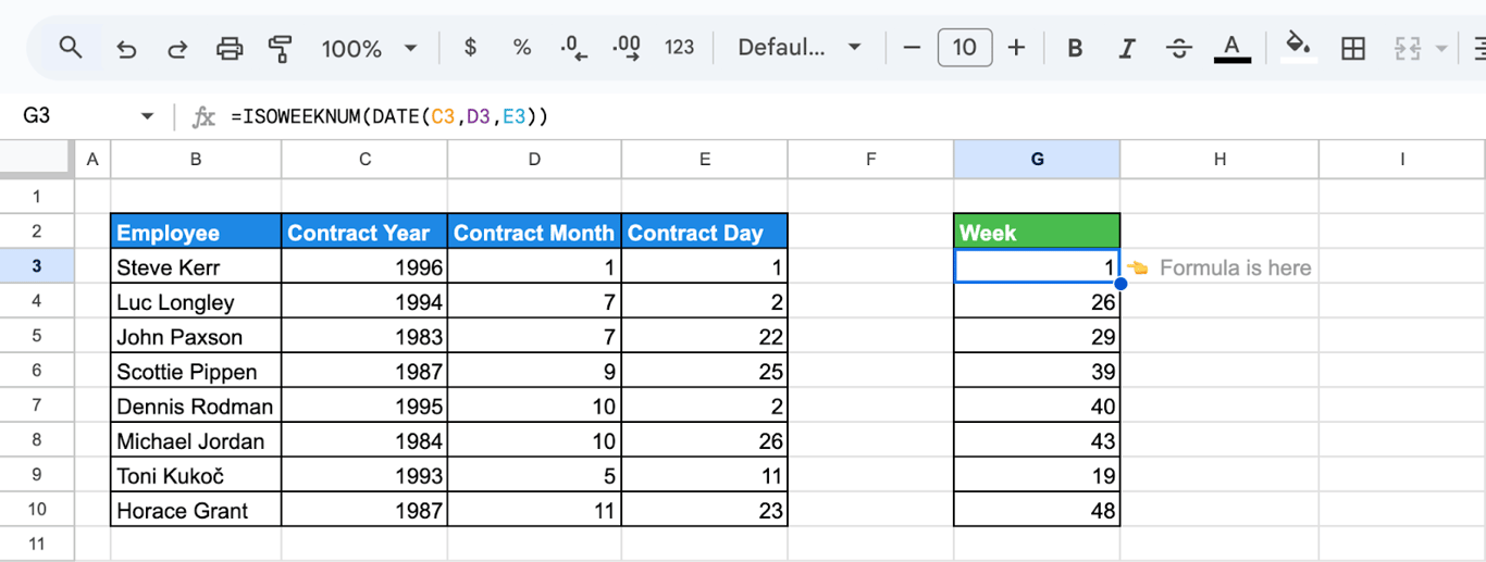
When year, month and day are stored in separate columns, the DATE function builds a date that WEEKNUM can use. With the contract start year in column C, the month in D and the day in E:
=WEEKNUM(DATE(C3, D3, E3))
Let’s break it down:
- DATE: combines the year, month, and day values into a complete date.
- WEEKNUM: calculates the corresponding week number for each date.
Combining ISOWEEKNUM with the DATE function
The same works for ISO weeks:
=ISOWEEKNUM(DATE(C3,D3,E3))
Let’s break it down:
- DATE: combine the year, month, and day values into a complete date.
- ISOWEEKNUM: determines the ISO week number for the constructed date.
The current week with ISOWEEKNUM and NOW
NOW returns the current date and time, so ISOWEEKNUM(NOW()) is the ISO week you are in today.

=ISOWEEKNUM(NOW())
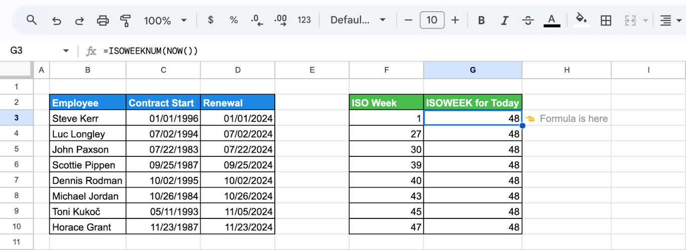
=ISOWEEKNUM(TODAY()) returns the same number. Compare it with the week of a deadline to see how many weeks are left.
Errors and wrong results in WEEKDAY and WEEKNUM
Errors and wrong results in WEEKDAY and WEEKNUM
#VALUE!: the cell is not a date
⚠️ Error: The function returns #VALUE! when the cell contains text instead of a date. A date that Google Sheets did not recognize is text: it sits on the left of the cell and does not change when you change the date format.
✅ Solution: Re-enter the date in a format the spreadsheet’s locale understands, or build it with DATE(year, month, day). For a column of text dates, DATEVALUE converts them.
#NUM!: the type is not valid
⚠️ Error: The function returns #NUM! when the type argument is a number it does not accept.
✅ Solution: Use 1, 2 or 3 for WEEKDAY, and 1, 2, 11 to 17 or 21 for WEEKNUM.
The day or the week is off by one
⚠️ Error: The result is a valid number, but not the one you expected.
✅ Solution: Check the type first: Sunday is 1 with the default and 7 with type 2. Then check how the date was read. In a month-first locale, 03/04/2026 is March 4; in a day-first locale it is April 3. Finally, make sure everyone uses the same week system, because WEEKNUM and ISOWEEKNUM can differ by one for the same date.
#N/A in a lookup that uses WEEKDAY
⚠️ Error: WEEKDAY and WEEKNUM do not return #N/A themselves, but a VLOOKUP or MATCH built on them does when the number is not in the lookup table.
✅ Solution: Make the type in the formula match the numbering in the table. A table numbered Monday = 1 needs WEEKDAY(date, 2).
Related Google Sheets functions
Related Google Sheets functions
Functions that are often used next to WEEKDAY and WEEKNUM, each with its own guide:
- UNIQUE: Extracts unique values from a range, removing duplicates to create a cleaner dataset.
- PIVOT: Creates dynamic summaries by grouping and aggregating data for easy analysis.
- IMPORTRANGE: Imports a range of cells from another spreadsheet.
- MATCH: Locates a value within a range and returns its relative position, aiding lookups.
- COUNTA: Counts non-empty cells in a range, useful for tracking entries or data completeness.
- MAX, MIN, MEDIAN: Identifies the highest value (MAX), lowest value (MIN), or middle value (MEDIAN) for statistical analysis.
- QUERY date filtering: Filters rows by a date or a date range inside a QUERY formula.
- MONTH/EOMONTH: Extracts the month from a date or returns the last day of a month, handy for monthly reports.
- Dates and times: Covers formatting, combining, splitting and sorting date and time values.
A week number is only as reliable as the dates behind it
A week number is only as reliable as the dates behind it
WEEKDAY and WEEKNUM do exactly what they are told with the dates they are given. Most wrong weekly reports are wrong earlier than that: dates pasted from an export as text, a file where day and month were swapped on import, a week that is missing because the export stopped on Thursday. The formula returns a tidy number either way.
The OWOX Data Marts extension for Google Sheets covers that half. A data analyst publishes a data mart (a table or an SQL query in your data warehouse) and makes it available for reports. In Sheets you open the extension, pick the data mart, tick the columns you want and run it. The rows land in a tab, ready for your formulas.
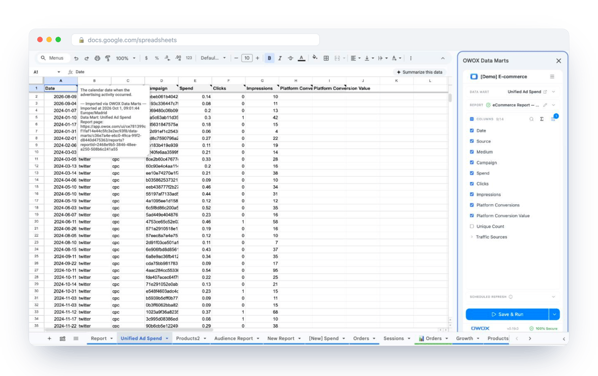
What changes for the person who maintains the sheet:
- Refresh replaces re-export. Refresh current report in the extension menu re-runs the same pull, and a scheduled refresh keeps the tab current without anyone touching it.
- The source is written on the sheet. The header cell of an imported tab carries a note with the data mart it came from, the time of the import and a link to the report.
- No SQL and no warehouse access needed. The analyst decides which data marts and columns are available. You choose from that list.
The extension does not write or change the analyst’s SQL, and WEEKNUM remains your tool for grouping by week. The dates arrive as real dates, from the same source every time, so the week they fall in is not a matter of who did the export. The extension comes with the OWOX Cloud plans of OWOX Data Marts; spreadsheet reporting describes both ways data reaches a sheet.
Turn your data into decisions.
Governed data marts give you the clean foundation ML needs to actually work.
- No AI hallucinations
- Analyst-governed definitions
- Every number traces to SQL
Frequently Asked Questions
Can I combine WEEKDAY with other functions to display weekday names?
Yes, you can combine WEEKDAY with functions like CHOOSE or VLOOKUP to display weekday names. For example:=CHOOSE(WEEKDAY(A1,1),"Sunday","Monday","Tuesday","Wednesday","Thursday","Friday","Saturday")This formula displays the weekday name for any given date.
How can I calculate the number of weeks between two dates in Google Sheets?
For full weeks between any two dates, divide the day difference by seven: =INT((B1 - A1) / 7). Subtracting week numbers, =WEEKNUM(B1) - WEEKNUM(A1), counts calendar weeks and only works when both dates are in the same year.
How can I add the word "Week" before the week number in Google Sheets?
Join the text to the week number with the & operator: ="Week " & WEEKNUM(A1). The result reads "Week 1", "Week 2" and so on. It is text, so keep a plain WEEKNUM column if you need to sort or calculate by week.
What should I do if my WEEKNUM function returns a #NUM! error?
WEEKNUM returns #NUM! when the type argument is not one it accepts. The valid types are 1 (week starts on Sunday), 2 (Monday), 11 to 17 (Monday through Sunday) and 21 (ISO weeks). If the date itself is text, the error is #VALUE! instead.
How do I calculate the ISO week number in Google Sheets?
To calculate the ISO week number, use the ISOWEEKNUM function. For example:=ISOWEEKNUM(A1)This formula assigns each date to its ISO-compliant week number, starting from the first Thursday of the year.
What is the difference between the WEEKDAY and WEEKNUM functions in Google Sheets?
The WEEKDAY function returns a number representing the day of the week for a specific date, with options to define the starting day (e.g., Sunday or Monday). The WEEKNUM function returns the week number of a specific date in a year, based on a chosen numbering system.