BigQuery Date Functions Explained

In the fast-paced world of data analytics, understanding how to manipulate and analyze dates in BigQuery is one such data warehouse that can significantly simplify your workflows and enhance data analysis. BigQuery's date functions are designed to offer powerful and flexible ways to work with dates, enabling you to perform a wide range of operations from basic date extraction to complex time-related calculations.

This guide will dive into the syntax, usage, and practical examples of essential BigQuery date functions, helping you master BigQuery data structure and date manipulations for more efficient data management and analysis.

Google BigQuery revolutionizes data analysis by offering immense processing capabilities, enabling easy handling of extensive datasets. This powerful tool is not just about the volume of data; it's about the speed and complexity of analysis it supports. For data analysts, becoming proficient with BigQuery's date and time data handling is crucial.

This proficiency allows for advanced data manipulation, facilitating accurate temporal analyses and the extraction of meaningful insights from sequences of chronological data. For instance, analyzing sales trends during specific holiday seasons or comparing quarterly revenue growth becomes straightforward with BigQuery's robust features.

The ability to swiftly perform such analyses without extensive data preprocessing or manual calculations makes BigQuery an invaluable asset for analysts looking to dive deep into temporal data trends.

At the core of Google BigQuery's features are its date-related functions, which stand as critical tools for any data analyst. These functions offer simplicity and efficiency in working with date and time data, covering a spectrum from basic operations like date extraction and formatting to more advanced calculations involving time intervals.

For example, functions like DATE_DIFF allow analysts to easily compute the difference between two dates, which is essential for tracking user retention or product lifecycle stages. Similarly, the DATE_TRUNC function can simplify the aggregation of data by periods (e.g., monthly or yearly sales analysis), enabling analysts to focus on trend identification and pattern analysis.

BigQuery's date functions empower analysts to conduct detailed temporal analyses, whether it's for performing cohort analyses, or making period-over-period comparisons, with unparalleled ease and precision.

BigQuery's date functions are indispensable tools for data analysts, offering nuanced control over date and time data. These functions enable a wide range of operations, from basic date extraction to complex temporal transformations with the help of SQL. Let's explore twelve essential date functions in BigQuery, complete with syntax and examples to guide you through their practical application.

The Current Date function is a straightforward yet powerful tool in BigQuery, designed to return the current date. This function is handy for appending date stamps on reports, performing date comparisons, and calculating time intervals from the present day back or forth. It ensures your data analyses remain relevant and time-accurate without hard-coding specific dates into your queries.

Syntax: CURRENT_DATE([timezone]);

• CURRENT_DATE is the function that returns the current date.
• [timezone] is an optional parameter that allows specifying the time zone for which the date should be returned. If omitted, the function uses the default time zone set in BigQuery, which is Coordinated Universal Time (UTC). This default setting ensures consistency in time-based data retrieval, regardless of the geographical location of the data analyst or the data source.

Example:

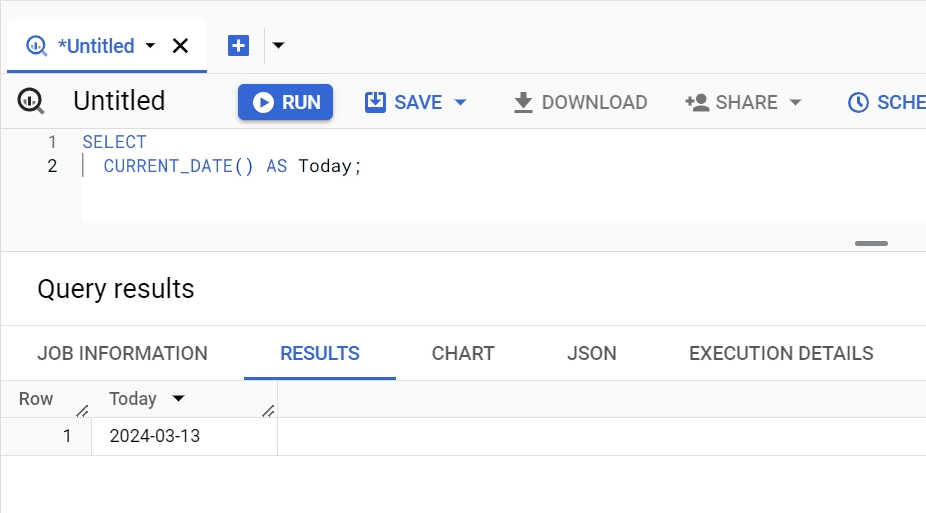
This example demonstrates how to retrieve the current date. If run on 2024-02-22, for instance, it would return "2024-02-22". This query is essential for dynamic reporting where the date of data retrieval is crucial. The AS Today part of the query renames the output column to "Today," making the result set clearer and more readable.

The DATE_ADD function is instrumental in calculating future dates by adding a specified interval to a given date. This function is invaluable for forecasting, setting deadlines, or scheduling future events based on current or specified dates. It simplifies temporal calculations, eliminating the need for cumbersome manual date adjustments.

Syntax: DATE_ADD(date, INTERVAL value date_part);

• DATE_ADD is the main instruction.
• date is the starting point from which the interval is added.
• INTERVAL value date_part specifies the quantity (value) and the type of interval (date_part, e.g., DAY, MONTH) to add to the date.

Example 1: Calculating a Date 30 Days in the Future. 

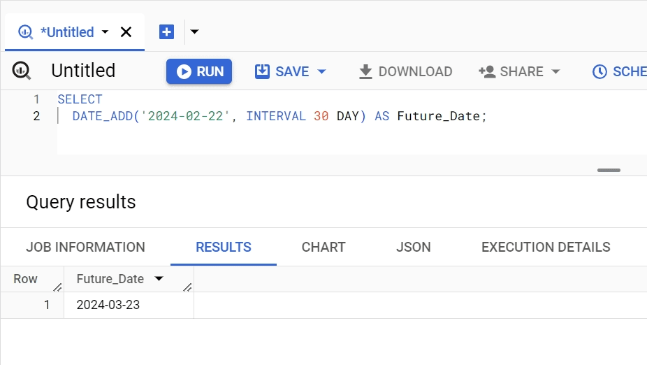
This query calculates the date 30 days after February 22, 2024, returning "2024-03-24". It's particularly useful for scenarios like calculating a payment due date that is 30 days from an invoice date. The AS Future_Date portion renames the output column for better clarity.

Example 2: Planning a Meeting 1 Week Ahead.

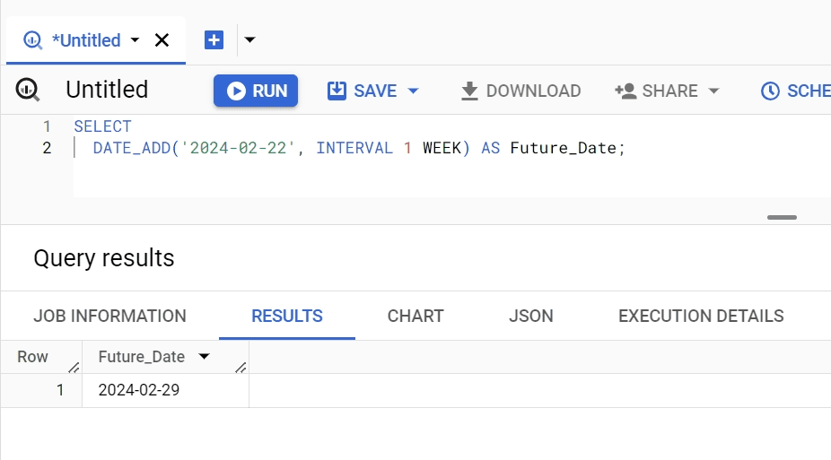
In this example, we're scheduling a meeting 1 week from February 22, 2024. The function returns "2024-02-29", providing a clear date for event planning or deadline setting. By specifying INTERVAL 1 WEEK, we demonstrate the versatility of the DATE_ADD function in handling various types of time intervals, making it equally effective for weekly planning.

By including examples with different intervals, such as days and weeks, this revised section aims to illustrate the flexibility and utility of the DATE_ADD function across a range of scenarios, enhancing its value in temporal calculations and planning activities.

The DATE_SUB function is the temporal counterpart to DATE_ADD, allowing users to compute past dates by subtracting a specified interval from a given date. This is beneficial for looking back into historical data, calculating expiration dates, or determining past deadlines.

Syntax: DATE_SUB(date, INTERVAL value date_part);

• DATE_SUB is the main instruction.
• date is the reference date from which the interval will be subtracted.
• INTERVAL value date_part defines how much time (value) and in what unit (date_part) will be subtracted from the date.

Example:

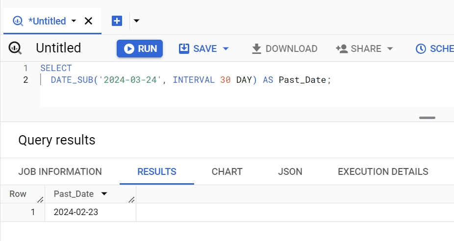
This example selects the date 30 days before March 24, 2024, which would be "2024-02-22". It's useful for scenarios like determining the date a month before a specific event. The renaming to Past_Date makes the output more intuitive.

The DATE_TRUNC function truncates a date to the specified component, such as the first day of the month or year, making it indispensable for monthly or yearly aggregations and comparisons.

Syntax: DATE_TRUNC(date_expression, date_part)

• DATE_TRUNC is the main instruction.
• date_expression is the date column or expression that you want to truncate.
• date_part specifies the component to which the date should be truncated, such as YEAR, ISO YEAR, QUARTER, MONTH, WEEK, ISO WEEK, DAY, etc.

Example:

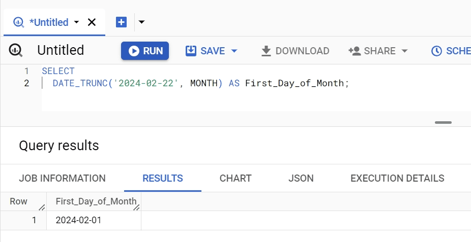
This query truncates the input date to the first day of its month, returning "2024-02-01". It's particularly useful for aligning dates to the start of their respective months for monthly reporting or analysis. The output column is aptly renamed to First_Day_of_Month for clarity.

The DATE_DIFF function is essential for calculating the difference between two dates, returning the interval in a specified unit, such as days, months, or years. This function is invaluable for measuring durations, aging reports, or tracking time elapsed between events. It offers a clear, quantitative insight into the temporal distance between two points in time.

Syntax: DATE_DIFF(date1, date2, date_part);

• DATE_DIFF is the main instruction.
• date1 is the first date (end date) in the comparison.
• date2 is the second date (start date) you're comparing the first date against.
• date_part specifies the unit for measuring the difference (e.g., DAY, MONTH).

Example:

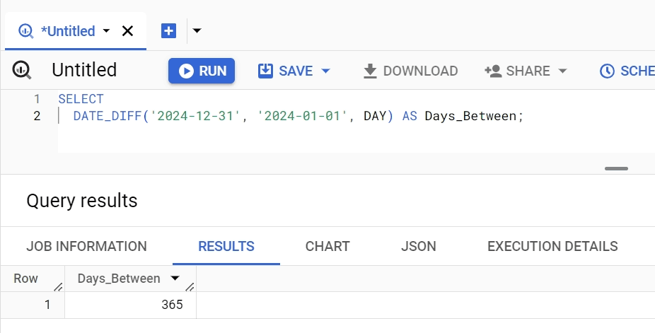
This example calculates the number of days between January 1, 2024, and December 31, 2024, which would return "365". This function is especially useful for calculating the tenure of an employee, the age of an account, or the duration between order placement and delivery. The result is named Days_Between for direct interpretation of the output.

The DATE_FROM_UNIX_DATE function converts a Unix date (the number of days since the Unix epoch, 1970-01-01) into a calendar date. This is particularly useful when working with Unix timestamps stored in datasets, enabling easy conversion to more readable date formats for analysis or reporting.

Syntax: DATE_FROM_UNIX_DATE(unix_date);

• DATE_FROM_UNIX_DATE is the main instruction.
• unix_date is an integer representing the number of days since 1970-01-01.

Example:

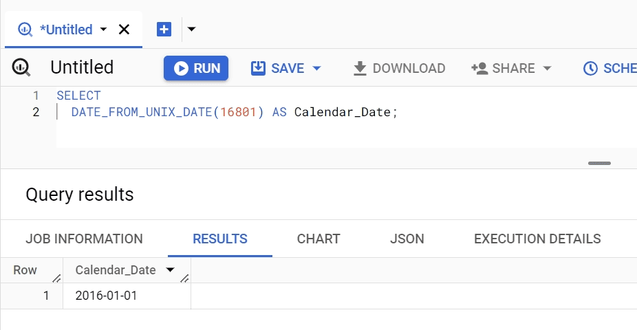
This query converts the Unix date 16801 into a calendar date, resulting in "2015-12-31". This function is critical when dealing with timestamps in Unix format, providing a straightforward method to transform them into human-readable dates. Calendar_Date serves as a clear column name for the resulting date value.

The LAST_DAY function returns the last day of the month, quarter, or year for a given date, facilitating end-of-period reporting, financial closing processes, or deadline calculations. It simplifies the process of identifying the final day of a specific time period without manual calculation.

Syntax: LAST_DAY(date, [date_part]);

• LAST_DAY is the main instruction.
• date is the input date from which the last day of the specified period will be calculated.
• [date_part] is an optional parameter that allows specifying the period like MONTH, QUARTER, or YEAR. If omitted, the default is MONTH.

Example:

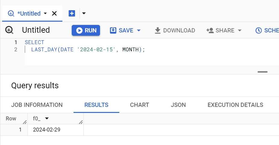
This example determines the last day of the month for February 15, 2024, which is "2024-02-29", considering 2024 is a leap year. The output, named Last_Day_of_February, clearly indicates the function's result, showcasing its utility in financial reporting where pinpointing the last day of a month or quarter is often crucial.

To illustrate the function's versatility, consider an example using the ISO WEEK interval: LAST_DAY('2024-02-15', 'ISO WEEK');

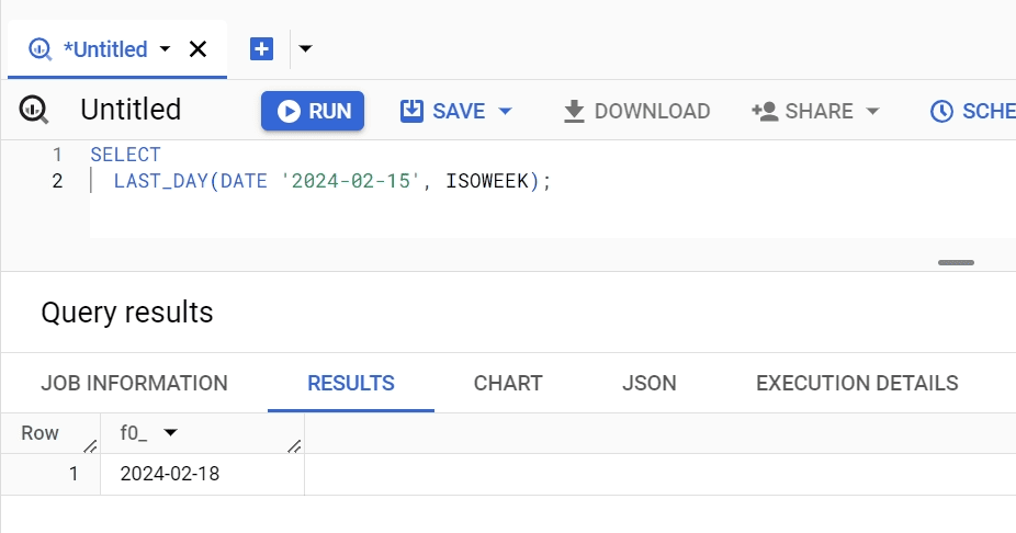
In this scenario, the query calculates the last day of the ISO week for February 15, 2024. Assuming that February 15 is a Thursday, the function returns "2024-02-18" as the last day of that ISO week. This example highlights how LAST_DAY can adapt to various intervals, providing flexibility in handling different types of period-end calculations.

The EXTRACT date function in BigQuery is a versatile tool designed to retrieve specific components from a date, such as the year, month, or day. This function is crucial when you need to analyze or categorize data based on time periods. It allows for more granular insights into trends and patterns by extracting and focusing on specific date elements.

Syntax: EXTRACT(part FROM date);

• EXTRACT is the main instruction.
• part specifies the component of the date you wish to extract, such as YEAR, MONTH, DAY, etc.
• date is the source from which the specified part should be extracted.

Example:

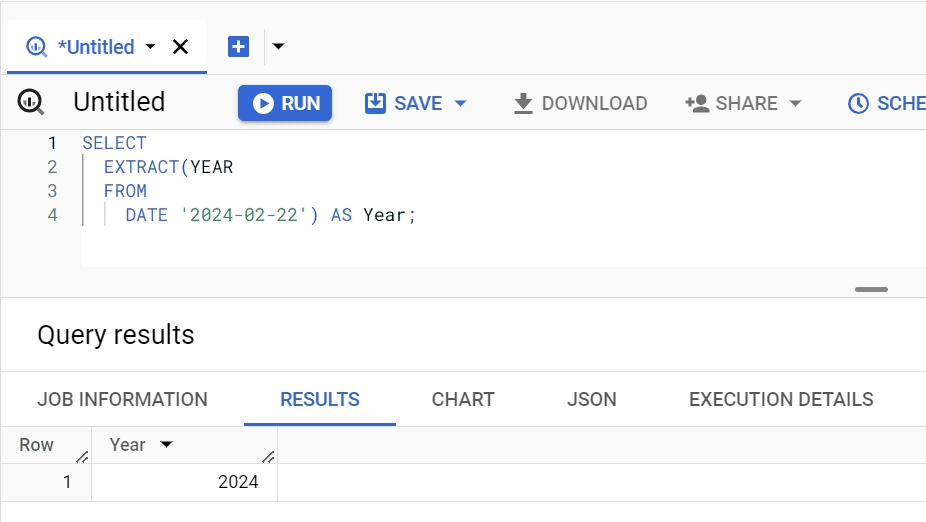
In this example, the function extracts the year component from the given date, returning "2024". This can be especially useful for aggregating sales data by year or for performing year-over-year growth analyzes. The result column is named Year for easy identification.

Expanding our exploration, consider the extraction of the week number from a date, an aspect that may not be as straightforward but is equally crucial for detailed temporal analysis: SELECT EXTRACT(WEEK FROM DATE '2024-02-22') AS WeekNumber;

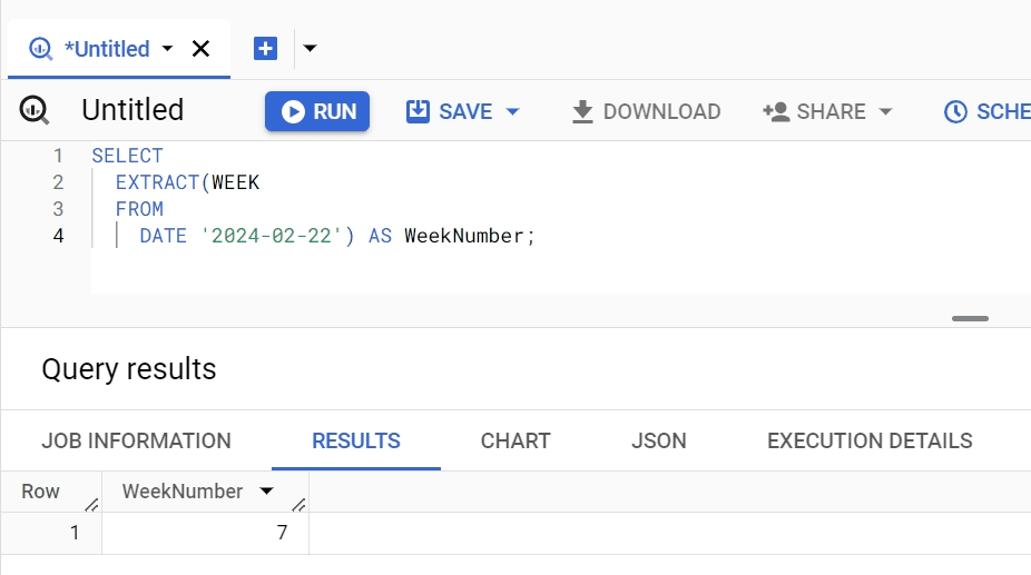
Here, the function extracts the week number from the given date, returning the specific week of the year. This example underscores the function's versatility, showcasing its utility in scenarios where understanding the distribution of events or data points within specific weeks of the year is essential.

The PARSE_DATE function converts a string into a date object based on a specified format. This is particularly useful when importing or integrating data from various sources where dates might be represented as strings. It ensures consistency in date format across your dataset, facilitating accurate comparisons and analyzes.

Syntax: PARSE_DATE(format, string);

• PARSE_DATE is the main instruction.
• format is a string that specifies the format of the input string, using format elements like %Y for year, %m for month, and %d for day. Additionally, when converting strings to date formats using PARSE_DATE, you must ensure that the order of elements (year, month, day, etc.) in your format string matches the order in your actual string data.
• string is the date string to be converted into a date object.

Beyond the basic date components (%Y, %m, %d), there are additional format elements you can use in BigQuery to handle other common variations in date string representations.

Here are some of these elements and their uses:

• %A: The full weekday name (English). Example: Wednesday
• %a: The abbreviated weekday name (English). Example: Wed
• %B: The full month name (English). Example: January
• %b or %h: The abbreviated month name (English). Example: Jan
• %C: The century (a year divided by 100 and truncated to an integer) as a decimal number (00-99). Example: 20
• %D: The date in the format %m/%d/%y. Example: 01/20/21
• %d: The day of the month as a decimal number (01-31). Example: 20
• %e: The day of the month as a decimal number (1-31); single digits are preceded by a space. Example: 20 (Note: BigQuery pads with zeros instead of spaces)
• %F: The date in the format %Y-%m-%d. Example: 2021-01-20
• %j: The day of the year as a decimal number (001-366). Example: 020
• %m: The month as a decimal number (01-12). Example: 01
• %Q: The quarter as a decimal number (1-4). Example: 1
• %U: The week number of the year (Sunday as the first day of the week) as a decimal number (00-53). Example: 03
• %u: The weekday (Monday as the first day of the week) as a decimal number (1-7). Example: 3
• %W: The week number of the year (Monday as the first day of the week) as a decimal number (00-53). Example: 03
• %w: The weekday (Sunday as the first day of the week) as a decimal number (0-6). Example: 3
• %x: The date representation in MM/DD/YY format. Example: 01/20/21
• %Y: The year with century as a decimal number. Example: 2021
• %y: The year without century as a decimal number (00-99), with an optional leading zero. Example: 21
• %%: A single % character. Example: %

For instance, if your format specifier is YYYY-MM-DD, your data string should be in the form 2024-03-15. If the order doesn't match, the function will not execute correctly, leading to errors.

Example:

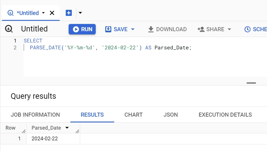
This query transforms a string representing a date into a date object, according to the specified format. Given the input string 2024-02-22, the PARSE_DATE function will parse this string as the 22nd day of February in the year 2024.

If you have a dataset with dates as strings in the format "YYYY-MM-DD", this function can standardize them into BigQuery date objects for further manipulation. The output is labeled Parsed_Date, providing clear identification.

The FORMAT_DATE is a function that converts a date object into a formatted string. This allows for the customization of how dates are presented in your reports or analyzes, making the data more understandable and tailored to your audience's expectations.

Syntax: FORMAT_DATE(format, date);

• FORMAT_DATE is the main instruction.
• format is a string that defines the desired output format, utilizing format specifiers such as %A for the full weekday name, %B for the full month name, and %d for the day of the month.
• date is the date object to be formatted.

Example:

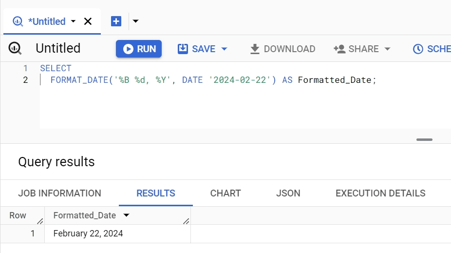
This example formats a date object into a more readable string, "February 22, 2024". This formatting is especially beneficial for generating user-friendly reports or when dates need to be displayed in a specific stylistic manner. The formatted date is aptly named Formatted_Date in the output.

The DATE function in BigQuery constructs a date from individual year, month, and day components. This function is crucial for creating specific dates within queries, allowing for precise date-based filtering, comparisons, and calculations.

Whether setting up historical data analyses, future projections, or simply needing to reference a particular date, the DATE function provides a straightforward method to generate exact dates based on provided values.

Syntax: DATE(year, month, day);

• DATE is the main function.
• year specifies the year component of the date.
• month indicates the month component, with 1 representing January and 12 representing December.
• day denotes the day component within the given month.

Example:

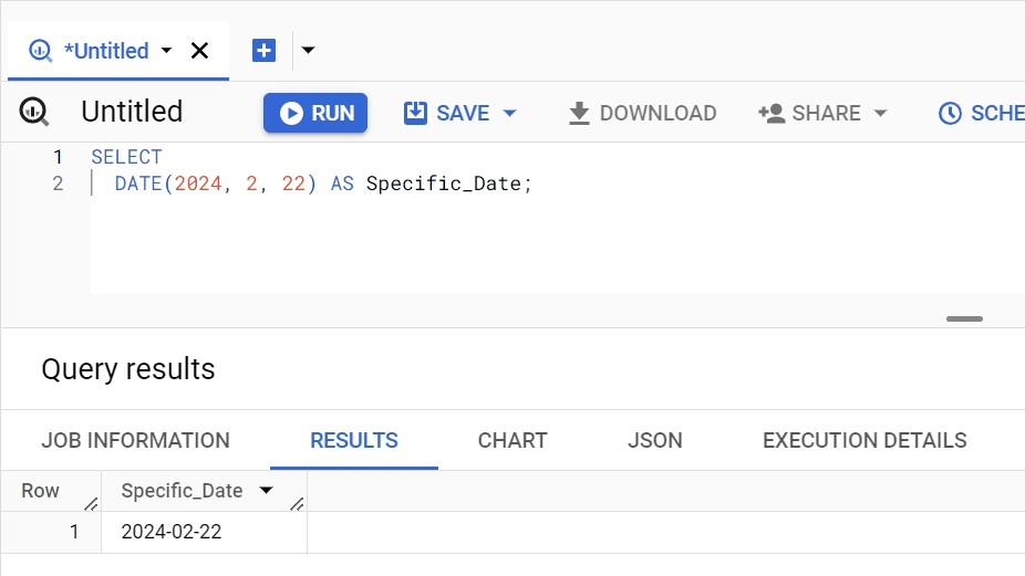
This query constructs a date for February 22, 2024. It is especially useful for scenarios where a specific date needs to be used for comparison, such as filtering records before or after this date. The AS Specific_Date part renames the output column, making the result set immediately understandable.

The UNIX_DATE function converts a DATE to the number of days since 1970-01-01, known as the Unix epoch. This function is valuable for when you need to perform operations that require date comparisons or calculations in a format that is agnostic of time zones or specific date formats. It simplifies the process of converting human-readable dates into a numeric format that is easily comparable and calculable within BigQuery.

Syntax: UNIX_DATE(date);

• UNIX_DATE is the main instruction.
• date is the DATE value to be converted into the Unix date format.

Example:

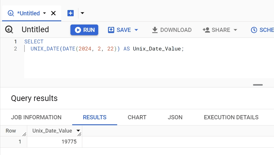
This example converts the specific date of February 22, 2024, into its corresponding Unix date value, representing the number of days since the Unix epoch. This numeric representation is mainly useful for calculating durations or differences between dates in a straightforward, format-agnostic manner. The AS Unix_Date_Value part of the query clearly labels the output, making the data easy to interpret.

Some general tips for using Date Functions in BigQuery would be to follow the below tips, these dive deeper into SQL template-level functionalities to help you optimize for better performance.

• Optimize Queries with Date Partitioning: For large datasets, use date partitioning. This optimizes queries by scanning only the relevant partitions, leading to faster performance and reduced costs.
• Employ EXTRACT for Component Retrieval and DATE_TRUNC for Precision: Utilize the EXTRACT function to isolate specific components (such as year, month, and day) from a date or timestamp. Integrate DATE_TRUNC to truncate a date or timestamp to a specified precision (e.g., the start of the month, year), facilitating analysis over uniform time intervals.
• Utilize DATE_ADD, DATE_SUB, and DATE_DIFF for Date Arithmetic: Perform date arithmetic such as adding or subtracting time intervals, or calculating differences between dates.
• Implement PARSE_DATE for Converting Strings: When working with string representations of dates or timestamps, use these functions to convert them into date or timestamp data types.
• Consider Time Zones with TIMESTAMP Functions: When manipulating TIMESTAMP data, be mindful of time zone conversions and use functions like TIMESTAMP_SECONDS, TIMESTAMP_MILLIS, etc., accordingly.
• Use CURRENT_DATE, CURRENT_DATETIME, and CURRENT_TIMESTAMP for Real-time Data: To capture the current date and time, use these functions, which can be particularly useful for logging and time-stamping operations.
• Regularly Update and Optimize Date Logic: As business logic evolves, regularly review and update the date manipulation logic in your queries to ensure they align with current requirements.
• Test Queries for Edge Cases: Especially around leap years, daylight saving time changes, and time zone quirks. This ensures the robustness of your data manipulation logic.
• Document Date Manipulation Logic: Document the purpose and function of date manipulations within your queries to aid in maintenance and understanding by other team members.

The LIMIT clause in SQL queries is used to specify the maximum number of rows that the query should return. This can be particularly useful in large datasets where you want to quickly preview or test your queries without processing the entire table.

However, relying too heavily on LIMIT for final analyses can skew your understanding of the data, as it may exclude relevant rows that could influence your insights. It's a powerful tool for managing query performance and costs in BigQuery, especially during the development and testing phases of your data analysis tasks.

Syntax: SELECT column_names FROM table_name LIMIT number;

• SELECT column_names: Specifies the columns to retrieve from the table.
• FROM table_name: Indicates the table from which to select the data.
• LIMIT number: Limits the number of rows returned by the query to a number.

Example:

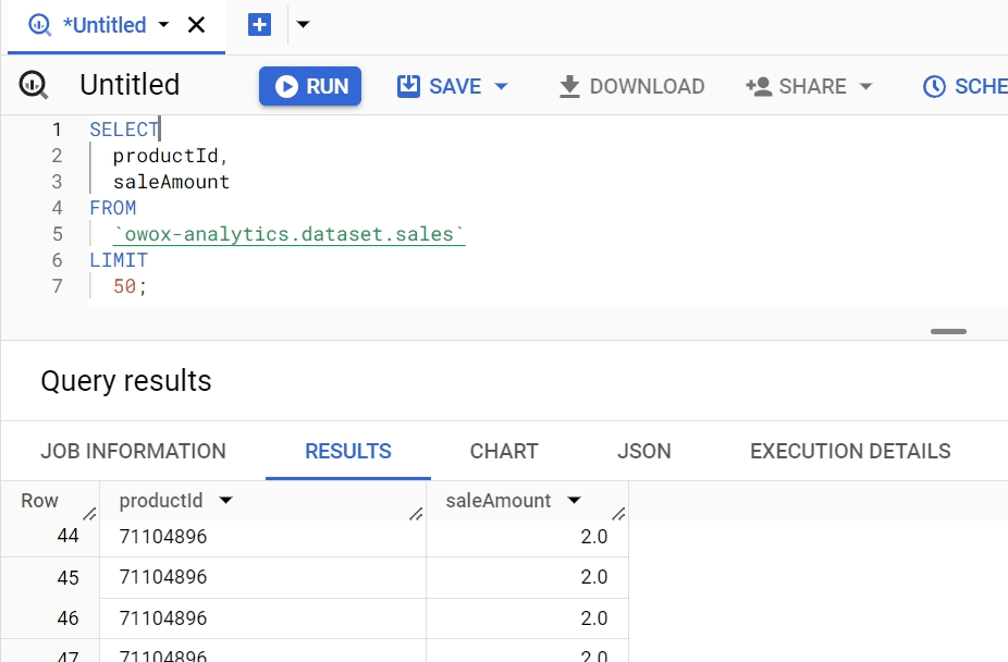
This query aims to fetch the first 50 rows from the sales table, focusing on productId and saleAmount. It's an efficient way to quickly check the data structure or perform a preliminary analysis without loading the entire dataset.

The use of LIMIT here speeds up the query execution by reducing the amount of data processed, making it ideal for testing query syntax or initial data exploration. However, for comprehensive analysis, removing the LIMIT clause to examine all relevant data is advisable to ensure accurate results.

When querying large datasets in BigQuery, it's efficient to retrieve only the columns you need. This practice minimizes the volume of data BigQuery needs to process, leading to quicker query execution and lower costs.

Especially in pay-per-query platforms like BigQuery, where costs are associated with the amount of data processed, selecting minimal columns can make a significant difference in optimizing resource usage and improving performance.

Syntax: SELECT column_names FROM table_name LIMIT number;

• SELECT needed_column: Directs BigQuery to fetch only the specified columns, rather than all columns in the table.
• FROM table_name: Specifies the table from which to retrieve the data.

Example:

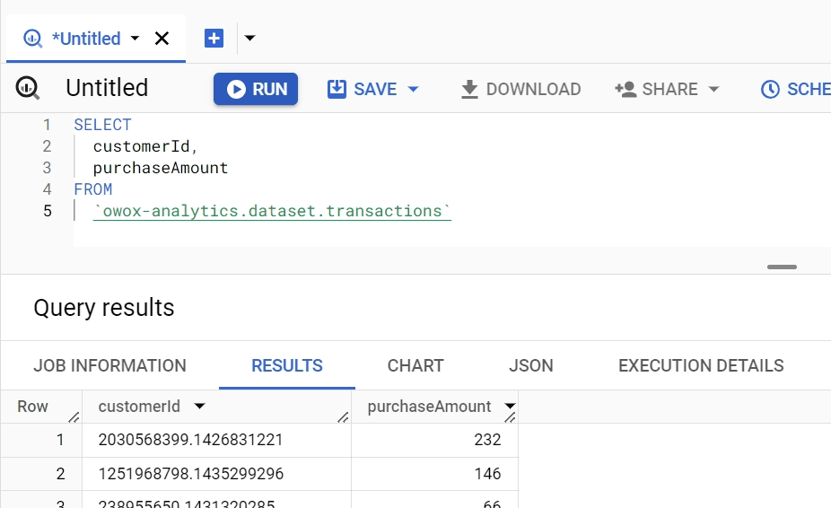
This query retrieves only the customerId and purchaseAmount columns from the transactions table. By doing so, it reduces the amount of data BigQuery needs to scan, especially useful if the table contains many other columns that are not relevant to the current analysis.

This selective approach to querying ensures that you're only dealing with the data you need, making subsequent processing, analysis, or visualization faster and more cost-effective. In contrast, using SELECT * would unnecessarily increase the query's cost and execution time by fetching all columns, regardless of their relevance to the analysis at hand.

EXISTS() is a logical function used to test for the existence of any record in a subquery. It returns TRUE if the subquery returns one or more records, and FALSE if the subquery returns no records. This function is often used in conditional statements within SQL queries, especially with WHERE clauses, to check if any rows satisfy the condition specified in the subquery.

COUNT() is an aggregate function that returns the count of items in a group. It can be used to count the number of rows in a table or the number of rows that match a specific condition. COUNT() is commonly used in SELECT statements along with GROUP BY clauses to aggregate data.

Using EXISTS() to check for the presence of rows corresponding to a specific condition in a subquery is more efficient than using COUNT(). This is because EXISTS() stops execution as soon as it finds the first match, thereby reducing processing time and resource usage. This method is notably useful for conditional checks in large datasets, improving performance by avoiding the full count of potentially large numbers of rows.

Syntax: SELECT column_names FROM table_name WHERE EXISTS (subquery);

• SELECT column_names: Specifies which columns to return from the outer query.
• FROM table_name: The table from which to select in the outer query.
• WHERE EXISTS: A condition that checks for the existence of rows returned by the subquery.
• (subquery): A separate query that returns rows based on a specific condition. If at least one row is returned, EXISTS evaluates to true.

Example:

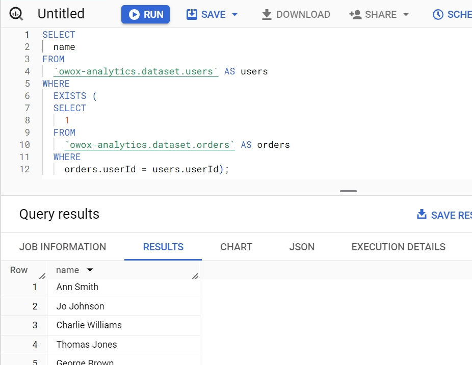
This example checks if any user in the users table has made an order. The subquery looks for orders matching each user's ID. If at least one order exists for a user, that user's name is selected. This method is faster than counting all orders for each user, especially beneficial in databases with extensive order histories.

Approximate aggregate functions, such as APPROX_COUNT_DISTINCT(), calculate a nearly accurate count of distinct values with less processing time compared to exact counts. This approach is useful in analytics where exact precision is not critical, but performance is, such as with large datasets where speed outweighs the need for absolute accuracy.

Syntax: SELECT APPROX_COUNT_DISTINCT(column_name) FROM table_name;

• SELECT APPROX_COUNT_DISTINCT(column_name): Calculates an approximate count of unique values for the specified column.
• FROM table_name: Specifies the table from which to retrieve the data.

Example:

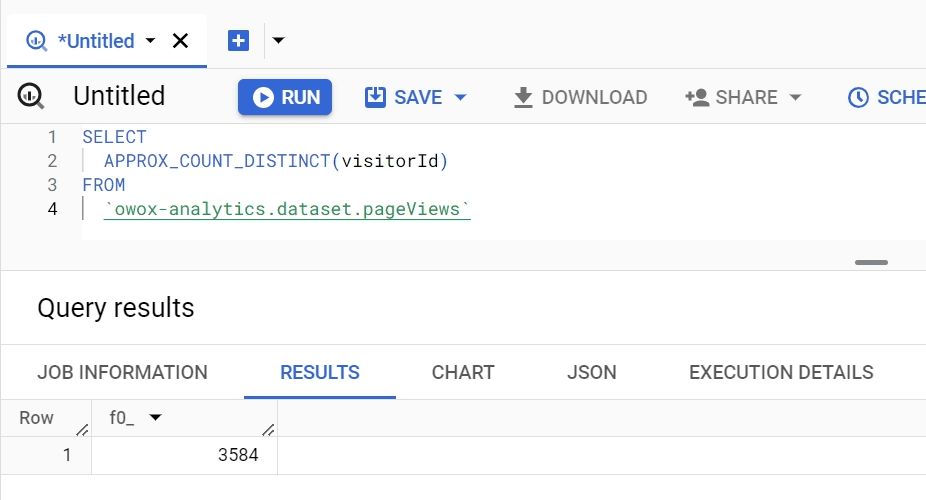
This query estimates the number of unique visitors by counting distinct visitorId values in the pageViews table. It's particularly useful for quickly assessing site traffic without incurring the computational cost of an exact count.

Window functions allow for complex calculations across sets of rows related to the current row without the need for self-joining tables. These functions can perform operations like running totals, averages, or rankings within a partition of the result set, offering a more efficient and readable approach to data analysis.

Syntax: SELECT column_name, AGG_FUNCTION(column_name) OVER (PARTITION BY column_name) FROM table_name;

• SELECT column_name, AGG_FUNCTION(column_name): Specifies the column to perform the aggregation on.
• OVER (PARTITION BY column_name): Defines the window over which the function operates. The partition clause divides the result set into partitions to which the function is applied.

Example:

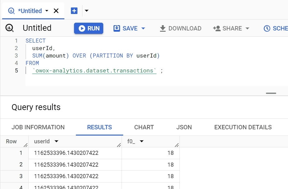
This query calculates the total transaction amount per user in the transactions table. Instead of using a self-join to aggregate transaction amounts for each user, it partitions the data by userId and sums the amount within each partition. This approach simplifies the query and improves performance by eliminating the need for complex joins.

In BigQuery, data processing efficiency can be significantly improved by optimizing the data types used in your queries, especially for operations like ORDER BY and JOIN.

INT64 is a data type used to represent integer values. It is part of BigQuery's standard SQL data types and is designed to hold 64-bit (or 8-byte) integer values. Using INT64 for these operations leverages BigQuery's storage and processing optimizations for integers, leading to faster query execution times. This practice is particularly beneficial when dealing with large datasets where performance can be a critical concern.

Syntax: SELECT * FROM table_name ORDER BY CAST(column_name AS INT64);

• SELECT * FROM table_name: Retrieves all columns from the specified table.
• ORDER BY: Orders the results based on the specified column.
• CAST(column_name AS INT64): Converts the column to an INT64 data type, optimizing the sort operation.

Example:

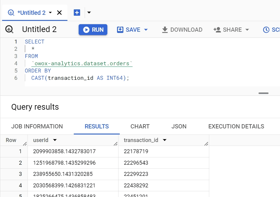
This query sorts the orders table by orderId after casting it to INT64. This ensures that the sorting operation is optimized for performance, making the query run faster, especially on large volumes of data.

Anti-joins are used to find rows in one table that do not have corresponding rows in another table. They are crucial for data analysis tasks that require identifying discrepancies or exclusions between datasets.

Some of the ways to optimize the use of Anti-joins would be to use NOT EXISTS or a LEFT JOIN with a WHERE IS NULL.

The NOT EXISTS operation is used with a subquery to test if no rows are returned by the subquery. It is commonly used in a WHERE clause. The NOT EXISTS approach is typically used to find records in one table that do not have a corresponding record in another table based on some join condition. The LEFT JOIN operation combined with a WHERE IS NULL clause is another way to achieve the same result.

A LEFT JOIN includes all records from the left table and the matched records from the right table, filling in with NULL where there are no matches. The WHERE IS NULL clause is then used to filter the results to only those records that did not have a match in the right table.

Using NOT EXISTS or a LEFT JOIN with a WHERE IS NULL clause for anti-joins can be more efficient than other methods, as they allow the query to stop processing as soon as the condition is met, rather than scanning entire tables.

Syntax: SELECT column_names FROM table_a WHERE NOT EXISTS (SELECT 1 FROM table_b WHERE table_a.id = table_b.id);

• SELECT column_names FROM table_a: Selects the desired columns from the first table.
• WHERE NOT EXISTS: Specifies that the query should return rows where no matching rows exist in the subquery.
• (SELECT 1 FROM table_b WHERE table_a.id = table_b.id): The subquery checks for the existence of matching rows in the second table.

Example:

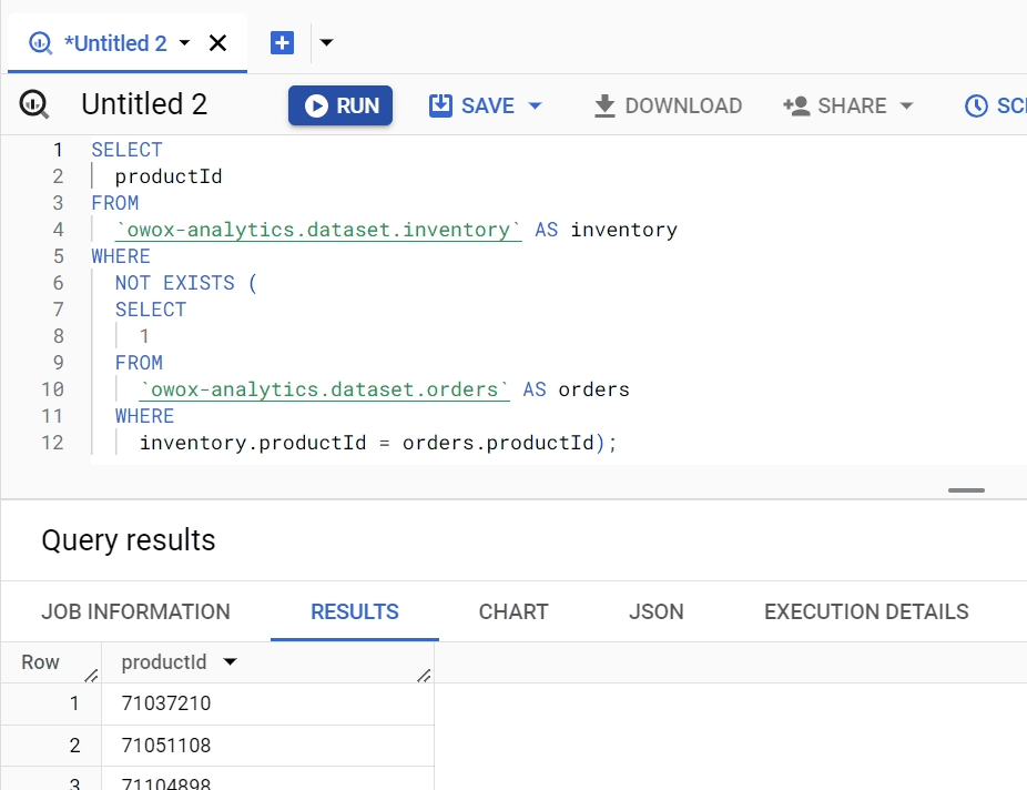
This query identifies products in the inventory that have not been ordered. The use of NOT EXISTS makes this operation efficient by quickly excluding matched records.

Regularly removing old or irrelevant data from your datasets can dramatically improve query performance and reduce storage costs. This practice, known as data trimming or pruning, ensures that your datasets remain relevant and manageable over time. It's particularly important in dynamic environments where data accumulates quickly.

Syntax: DELETE FROM table_name WHERE condition;

• DELETE FROM table_name: Specifies the deletion operation from the given table.
• WHERE condition: Defines the criteria for which rows should be deleted

Example:

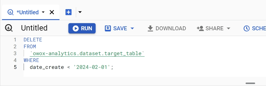
This command removes all log entries in the logs table that are older than January 1, 2023. Regular execution of such queries helps in maintaining optimal table size and improving the efficiency of data retrieval and analysis operations.

The order in which conditions are placed in the WHERE clause can significantly impact query efficiency. By positioning the most restrictive conditions first, BigQuery can quickly reduce the dataset size, leading to faster query execution. This strategy leverages BigQuery's ability to discard irrelevant data early in the processing stage, optimizing resource use and minimizing processing time.

Syntax: SELECT column_names FROM table_name WHERE most_restrictive_condition AND less_restrictive_condition;

• SELECT column_names: Specifies the columns to retrieve.
• FROM table_name: Identifies the table from which to select data.
• WHERE most_restrictive_condition AND less_restrictive_condition: Filters the data, starting with the condition that eliminates the most rows.

Example:

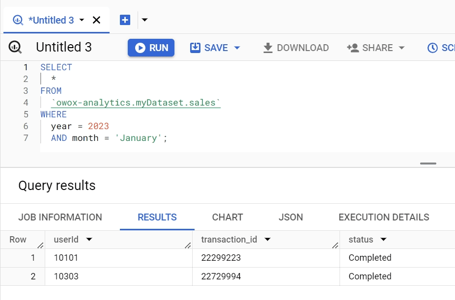
This query first filters the sales table by the year, likely a more restrictive condition than the month, thereby reducing the amount of data processed in subsequent operations.

Partitioning and clustering are BigQuery features that organize data into more manageable segments. Partitioning divides the table based on a specific key, such as a date, allowing queries to scan only relevant partitions. Clustering further sorts data within each partition, optimizing queries that filter on clustered columns. Together, they enhance query performance by limiting the amount of data scanned.

Syntax: CREATE TABLE table_name PARTITION BY DATE(date_column) CLUSTER BY cluster_column AS SELECT * FROM source_table;

• CREATE TABLE table_name: Creates a new table.
• PARTITION BY DATE(date_column): Specifies the column to partition the table by.
• CLUSTER BY cluster_column: Specifies the columns to cluster data within the partitions.
• AS SELECT * FROM source_table;: Defines the data to populate the new table.

Example:

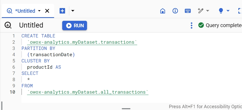
This creates a transactions table partitioned by transactionDate and clustered by productId, optimizing queries filtered by these columns.

The ORDER BY clause in BigQuery SQL is used to sort the result set of a query by one or more columns. It can sort the data in ascending order (which is the default) or descending order. The ORDER BY clause is an essential part of SQL queries when you need the results to be returned in a specific order.

Sorting data with ORDER BY is resource-intensive. By deferring this operation until after filtering (WHERE) and aggregation (GROUP BY), you can significantly reduce the computational load. This approach processes a smaller subset of data, thereby speeding up the query.

Syntax: WITH FilteredData AS (SELECT * FROM table_name WHERE condition) SELECT * FROM FilteredData ORDER BY column_name;

• WITH FilteredData AS (...): Creates a temporary filtered dataset.
• SELECT * FROM FilteredData: Selects the data from the temporary dataset.
• ORDER BY column_name;: Applies sorting to the reduced dataset.

Example:

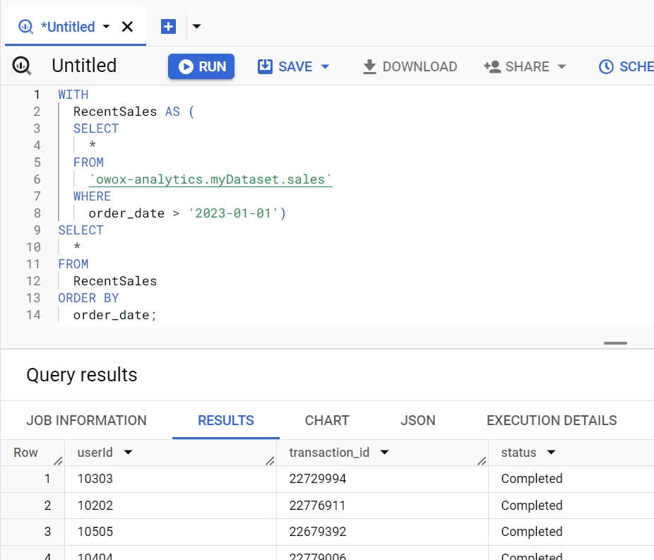
This filters the sales data for recent entries before sorting them by saleDate, enhancing performance by sorting a smaller data set.

The SEARCH function in BigQuery checks to see if a search query matches any part of a document using an optional text analyzer. It returns TRUE if there is a match based on the specified or default text analyzer and FALSE otherwise. This function is particularly useful for implementing full-text search features directly within BigQuery SQL queries.

Syntax: SELECT * FROM table_name WHERE SEARCH (column_name, 'search_term');

In the section:

• FROM table_name: Specifies in which table it needs to search.
• column_name: The name of the column in your table where you want to search for the text. This specifies the field that the search operation targets.
• 'search_term': The string or text expression you are looking for within the specified column. This would be the pattern or exact text you're trying to match.

The function can be used in the WHERE clause of a SQL query to filter rows based on whether the specified column contains the search term.

Example:

Let's say you have a dataset of customer feedback stored in a table named customer_feedback, and you want to find all feedback that mentions "excellent service". The column where this text might be found is named feedback_text.

Using the conceptual SEARCH() function, the query would look something like this:

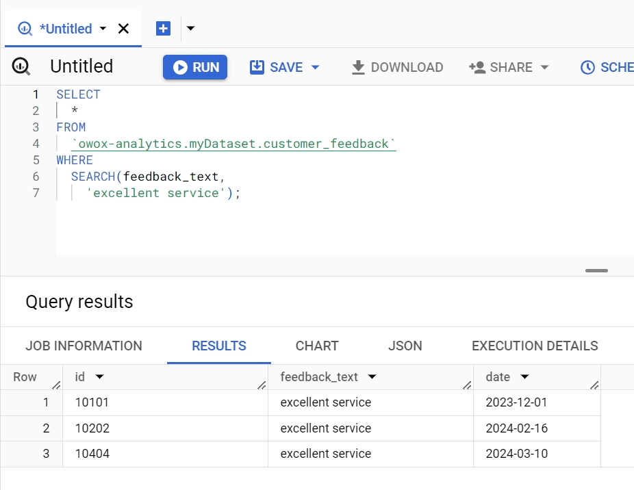
Here:

• SELECT *: This selects all columns from the rows where the condition is met, meaning you get the full records of customer feedback that match your search criteria.
• FROM customer_feedback: Indicates the table you are querying, which in this case contains customer feedback data.
• WHERE SEARCH(feedback_text, 'excellent service'): Filters the rows to only those where the feedback_text column contains the phrase "excellent service". The SEARCH() function here is used to efficiently locate these instances within potentially large volumes of text data.

BigQuery caches query results for 24 hours, which can be leveraged for repeated queries to save cost and time, especially for dashboards and reports. Automatically applied to queries where the SQL and dataset haven’t changed, no specific syntax is needed.

By applying these strategies, you can significantly enhance the efficiency and performance of your queries in BigQuery, ensuring faster data retrieval and analysis while managing computational resources effectively.

Encountering format inconsistencies or data type errors with date functions fall under common issues. These issues often stem from incorrect syntax or misunderstanding the function's requirements. Familiarizing yourself with BigQuery's documentation and error messages can guide you in resolving these challenges.

Incorrect date formatting in source data (e.g., CSV files) can lead to errors when BigQuery attempts to interpret dates, resulting in failed data loads or incorrect queries.

✅ Solution:

To address the issue of date format inconsistencies in source data, it's crucial to understand how to correctly format dates for BigQuery to ensure successful data loads and accurate queries.

BigQuery expects date and datetime values to be in specific formats:

• Dates should be in YYYY-MM-DD format.
• Timestamps (dates with time information) should adhere to the YYYY-MM-DDTHH:MM:SS.SSSZ format, which is an ISO 8601 format.

When data does not match these formats, BigQuery may not interpret dates correctly, leading to errors. To resolve this, you can use BigQuery's functions like PARSE_DATE for dates and PARSE_TIMESTAMP for timestamps to convert strings into the correct date or timestamp format.

Queries might fail or return unexpected results when dates fall outside valid ranges, such as querying "February 30th".

✅ Solution:

When dealing with dates in SQL or specifically in BigQuery, ensuring that date values are valid is crucial to prevent queries from failing or returning unexpected results. Invalid date ranges, such as "February 30th", can cause such issues.

To handle these effectively, BigQuery provides a function called SAFE.PARSE_DATE, designed to parse a string into a DATE value safely without causing an error for invalid dates.

Syntax: SAFE.PARSE_DATE(format, string);

This function attempts to convert a string into a DATE value based on the specified format. The format parameter determines how the function interprets the string, using format elements like %Y for the year, %m for the month, and %d for the day. If the string doesn't match the format or represents an invalid date, the function returns NULL instead of raising an error.

• Format: A string that specifies the format of the date in the string parameter. This format must match the structure of the date in the string, using specific format elements.
• String: The string that you want to convert into a DATE value.

Example Application:

Consider a scenario where you're querying a dataset that includes a column with date strings, and you're not sure if all date strings represent valid dates. You can use SAFE.PARSE_DATE to safely parse these strings into DATE values, ensuring that your query does not fail due to invalid dates.

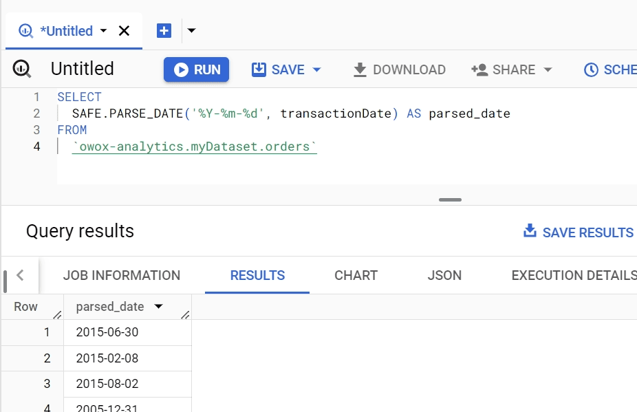
In this example:

• %Y-%m-%d is the format parameter, indicating that the date string is expected to be in the format of "year-month-day", such as "2024-02-26".
• date_string is the column that contains the date strings you want to convert into DATE values. This could be any column in your dataset that stores date information in string format.
• SAFE.PARSE_DATE is applied to each value in the date_string column, attempting to parse it into a DATE. If a string is an invalid date or does not match the specified format, the function returns NULL for that value instead of causing the query to fail.

This approach ensures that your query can handle date strings gracefully, converting valid dates to DATE values while ignoring invalid dates, thus maintaining the integrity of your query execution process.

The DATE_DIFF function requires both arguments to be of the DATE data type. Using a DATETIME or TIMESTAMP can lead to errors.

✅ Solution:

The DATE_DIFF function is used to calculate the difference between two dates, returning the number of days from the first date to the second date. To use it correctly, it's crucial that both arguments are of the DATE data type. If the arguments are of the DATETIME or TIMESTAMP data types, you'll encounter errors due to type mismatch.

We have discussed above in detail about this function and how you can use it effectively.

Attempting to use DATE_DIFF with an unsupported date part (e.g., SECOND) results in an error, as DATE_DIFF is designed to work with date parts like DAY, MONTH, and YEAR.

✅ Solution:

When dealing with date and time calculations in SQL or similar query languages, understanding the syntax and application of functions like DATE_DIFF, DATETIME_DIFF, TIMESTAMP_DIFF, or TIME_DIFF is crucial. These functions are designed to calculate the difference between two dates or timestamps, but they vary in the granularity of time they support.

NOTE: We have discussed the DATE_DIFF function in detail previously in this article.

Syntax: TIMESTAMP_DIFF(timestamp1, timestamp2, date_part)

This function is used for timestamp values, supporting even more granular differences, including SECONDS.

Example Application:

Imagine you have two timestamps: timestamp1 = '2023-01-01 12:01:10' and timestamp2 = '2023-01-01 12:00:00'. You want to calculate the difference in seconds between these two timestamps.

Using TIMESTAMP_DIFF, the syntax would be: SELECT TIMESTAMP_DIFF(TIMESTAMP '2023-01-01 12:01:10', TIMESTAMP '2023-01-01 12:00:00', SECOND) AS difference_in_seconds

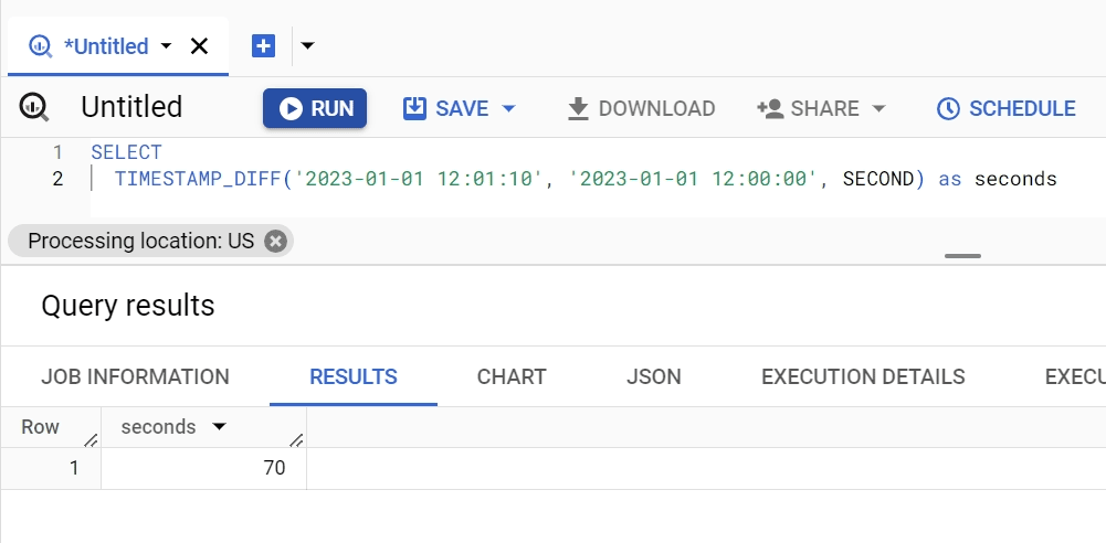
This function will return the difference in seconds between timestamp1 and timestamp2. In this case, the output would be 70 seconds, showing the exact duration between these two points in time.

Explanation:

• TIMESTAMP_DIFF(): This is the function used to calculate the difference between two timestamps.
• TIMESTAMP '2023-01-01 12:01:10': The first argument to TIMESTAMP_DIFF, representing the first timestamp. You need to use the TIMESTAMP keyword to explicitly cast the string to a timestamp. This is your timestamp1.
• TIMESTAMP '2023-01-01 12:00:00': The second argument, represents the second timestamp. Similar to the first timestamp, you use the TIMESTAMP keyword to cast the string. This is your timestamp2.
• SECOND: The third argument to TIMESTAMP_DIFF, specifies that you want the difference in seconds.
• AS difference_in_seconds: This part of the query renames the output of the TIMESTAMP_DIFF function to difference_in_seconds for clarity.

Syntax: TIME_DIFF(time_expression1, time_expression2, date_part)

• time_expression1 and time_expression2 are the two times you want to compare.
• date_part is the unit in which you want the result (e.g., HOUR, MINUTE, SECOND).

Example Application:

Imagine you want to calculate the difference in minutes between two times: 08:00:00 and 09:30:00. You would use the TIME_DIFF() function as follows:

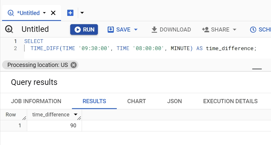
This query will return 90, indicating that there is a 90-minute difference between 09:30:00 and 08:00:00.

Explanation:

• TIME '09:30:00': The first argument to TIME_DIFF(). It represents the first time point, 9:30 AM, specified as a TIME literal. In the context of this function, this is considered the "end time."
• TIME '08:00:00': The second argument to TIME_DIFF(). It represents the second time point, 8:00 AM, also specified as a TIME literal. This is considered the "start time" for the purpose of the calculation.
• MINUTE: The third argument specifies the unit in which the time difference should be calculated and returned. In this case, MINUTE is used, indicating that the result will express the difference in minutes.
• AS time_difference: This part of the query aliases the result of the TIME_DIFF() function as time_difference. This alias is what the column containing the result of the computation will be named in the output.

This approach is particularly useful in scenarios requiring precise time calculations, such as in logging events, measuring durations, or scheduling tasks in databases and applications.

The DATE_TRUNC function expects a DATE argument, but receiving a TIMESTAMP or DATETIME triggers a type error.

✅ Solution:

It's important to ensure that the data type of the input argument matches what the function expects. Typically, DATE_TRUNC requires a DATE data type, but if you're working with a TIMESTAMP or DATETIME, you must explicitly cast these to DATE to avoid type errors.

Syntax: DATE_TRUNC(date_expression, 'precision')

• A date_expression in BigQuery is an expression that evaluates to a DATE value.
• The 'precision' specifies the level of truncation, such as 'day', 'month', 'year', etc. The date_expression is the date or timestamp value you want to truncate. If date_expression is a TIMESTAMP or DATETIME, it must be cast to DATE.

CAST(date_expression AS DATE)

• This is the syntax for casting a TIMESTAMP or DATETIME to a DATE. It converts the input into a DATE format, ensuring compatibility with DATE_TRUNC's requirements.

Example Application:

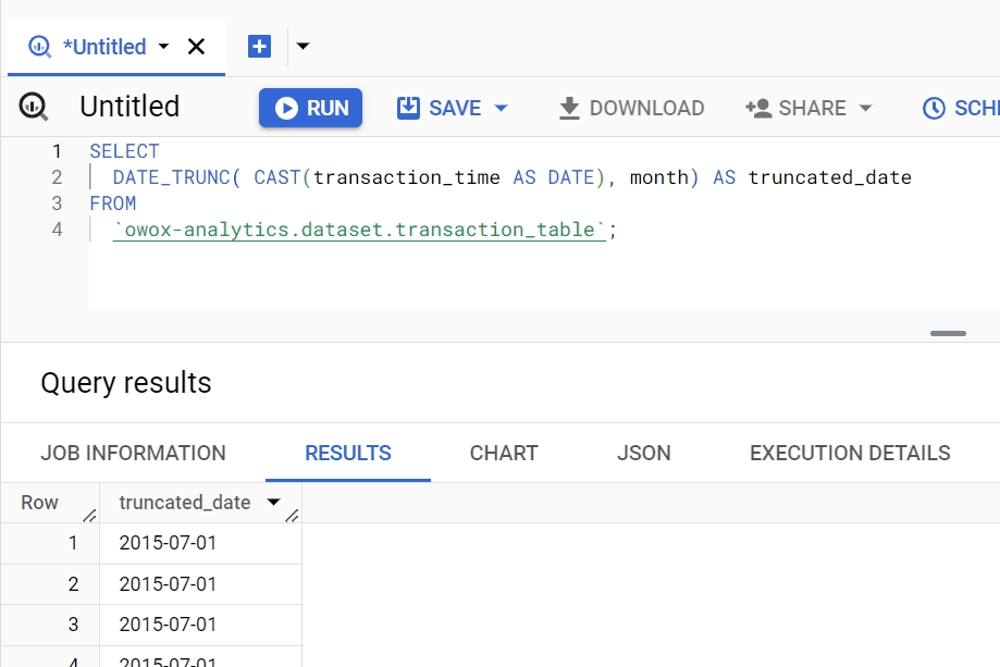
In this example, timestamp_column is assumed to be of the TIMESTAMP or DATETIME data type. The CAST function converts timestamp_column to a DATE type. Then, DATE_TRUNC truncates this date to the first day of the month that the original timestamp falls into, effectively grouping your data by month.

• DATE_TRUNC(..., month) truncates the converted date to the first day of the month it belongs to.
• CAST(timestamp_column AS DATE) ensures the timestamp is treated as a simple date, stripping the time component.
• AS truncated_date names the output column for easier reference.

This approach is useful for analyzing trends over time, allowing you to aggregate and compare data on a monthly basis without concern for the specific days or times events occurred.

Aggregating data by dates without proper grouping or using incorrect functions can lead to misleading results.

✅ Solution:

Aggregating data by dates involves summarizing or combining values from multiple data entries based on their date attributes, crucial for analyzing trends over time, understanding seasonal patterns, or making forecasts. However, without proper grouping or using incorrect functions, the aggregation can yield misleading results.

Here's a breakdown of how to approach this task correctly, focusing on the syntax components and an example application.

Syntax Components:

1. Aggregation Functions: These are functions like SUM(), AVG(), COUNT(), MAX(), and MIN() that aggregate multiple values into a single value. Choosing the right aggregation function is critical based on whether you're summing values, finding averages, counting entries, etc.
2. GROUP BY Clause: This SQL clause groups rows that have the same values in specified columns into summary rows. When aggregating data by dates, you'll often group by the date column or parts of it (like year or month).
3. EXTRACT Function: This function is used to retrieve specific parts of a date, such as a year, month, or day. It's particularly useful for grouping data by these components, allowing for more granular or specific aggregations over time.

Example Application:

Imagine you have a database of sales transactions, and you want to calculate the total sales per month. Here's how you might approach this:

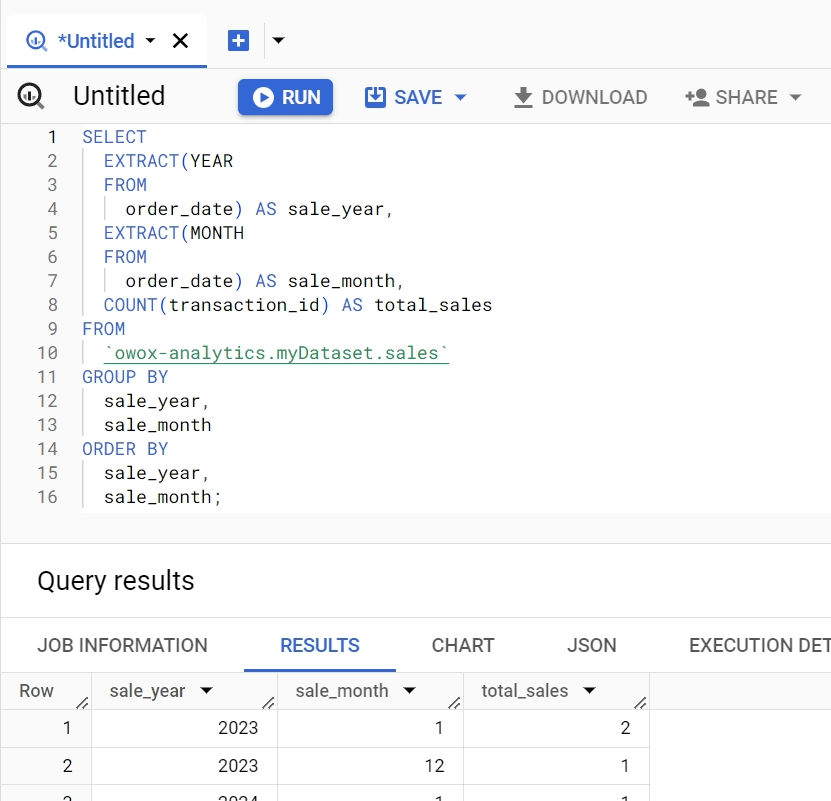
Example Explanation:

• EXTRACT Function: We extract the year and month from the sale_date column to use for grouping. This allows us to aggregate sales data on a monthly basis across multiple years.
• COUNT Function: We use COUNT(transaction_id) to calculate the total sales for each group (each unique year and month combination).
• GROUP BY Clause: We group the results by sale_year and sale_month, which are the extracted year and month from the sale_date. This ensures that our aggregation is accurate and meaningful, reflecting the total sales for each month.
• ORDER BY Clause: Finally, we order the results by sale_year and sale_month to present the data in chronological order, making it easier to analyze trends over time.

This approach ensures accurate and insightful aggregation of sales data by date, allowing for effective analysis of monthly sales trends.

Complex date manipulations or operating on large datasets without optimization can lead to slow query performance.

✅ Solution:

To address performance issues with date functions, especially when dealing with complex date manipulations or large datasets, it's crucial to understand and apply optimization techniques in Google BigQuery. Here, I'll break down the syntax components related to partitioning, clustering, and efficient use of date functions, followed by an example to illustrate these concepts in action.

Syntax:

1. Partitioning: Partitioning divides your table into segments, making queries more efficient by scanning only relevant partitions. You can partition tables based on a date or timestamp column.

Syntax for creating a partitioned table: 

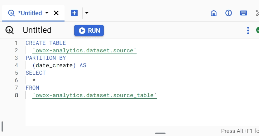
2. Clustering: Clustering orders the data within each partition. When combined with partitioning, it further reduces the cost and increases the speed of queries by focusing on a more specific subset of data.

Syntax for creating a clustered table:

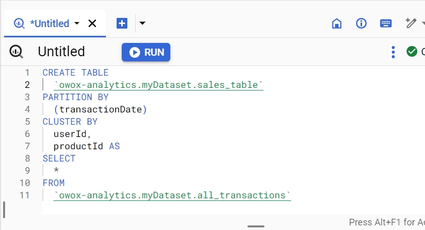
3. Minimizing Complex Date Functions: Avoid using complex date functions on large datasets directly. Instead, pre-compute these values or simplify your queries.

Example of simplifying a query:

Instead of doing the following:

Pre-compute the year in a column or simplify as:

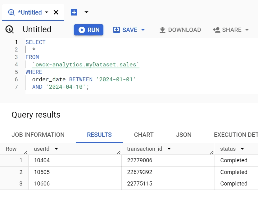
Example Application:

Suppose you have a large dataset with sales transactions, and you frequently query the data to analyze monthly sales performance. The table is partitioned by the transaction date and clustered by product and region to optimize performance.

Example Explanation:

• Partitioning by transaction_date: This ensures that queries filtering by date only scan the relevant partitions, reducing the amount of data read and thereby speeding up the query.
• Clustering by product_id and region_id: Within each date partition, data is organized based on product and region, making queries filtered by these columns much more efficient as they can skip irrelevant data.
• Use case: When querying for total sales of a specific product in a specific region for a certain month, BigQuery scans only the data for that month (due to partitioning) and quickly locates the relevant product and region (due to clustering), significantly reducing the query's execution time and cost.

By following these practices – leveraging partitioning and clustering based on date columns and minimizing the use of complex date functions, you can optimize query performance in BigQuery, especially when working with large datasets or performing intricate date manipulations.

If you want to improve your Google BigQuery skills, consider diving deeper into mastering these advanced functions for more comprehensive data analysis.

• Conversion Functions: In BigQuery, conversion functions assist in changing data types from one form to another, improving data compatibility and simplifying analysis.

• Array Functions: BigQuery’s array functions enable the processing and manipulation of arrays in your data sets, supporting intricate data operations.

• Aggregate Functions: Aggregate functions in BigQuery calculate collective values from your data, which are crucial for detailed statistical analysis.

• DML (Data Manipulation Language): DML commands in BigQuery, including INSERT, UPDATE, DELETE, and MERGE, facilitate effective alterations to the data within your tables.

• String Functions: String functions in BigQuery help you manipulate text data through operations such as concatenation, substring extraction, and pattern matching, enhancing your data handling capabilities.

Integrating the OWOX BI BigQuery Reports Add-on into your data analysis workflow brings forth a multitude of benefits. This extension seamlessly connects with BigQuery, enabling automatic extraction and manipulation of date-related data. By taking advantage of its capabilities, analysts can effortlessly access and analyze vast datasets, empowering them to derive actionable insights swiftly and efficiently.

Moreover, the OWOX BI BigQuery Reports Extension facilitates comprehensive reporting, providing analysts with the tools needed to present data-driven findings effectively. Its intuitive interface and robust features empower users to create insightful reports tailored to specific business needs. By leveraging this extension, organizations can make informed decisions based on accurate data analysis, ultimately driving growth and success.