Standard SQL in Google BigQuery: Advantages and Examples of Use in Marketing

Oksana Litvenko, Digital Analyst @ OWOX

Liubov Zhovtonizhko, Creative Writer @ OWOX

Apr 20, 2019

In 2016, Google BigQuery introduced a new way to communicate with tables: Standard SQL. Until then, BigQuery had its own structured query language called BigQuery SQL (now called Legacy SQL).

At first glance, there isn’t much difference between Legacy and Standard SQL: the names of tables are written a little differently; Standard has slightly stricter grammar requirements (for example, you can’t put a comma before FROM) and more data types. But if you look closely, there are some minor syntax changes that give marketers many advantages.

Move your marketing data into BigQuery automatically without SQL and developers. OWOX BI is the easiest way to collect and blend all marketing data in a single storage. No experience in coding needed.

BOOK A DEMO

What are the advantages of Standard SQL over Legacy SQL?

New data types: arrays and nested fields

Standard SQL supports new data types: ARRAY and STRUCT (arrays and nested fields). This means that in BigQuery, it has become easier to work with tables loaded from JSON/Avro files, which often contain multi-level attachments.

A nested field is a mini table inside a larger one:

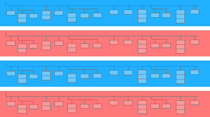
In the diagram above, the blue and red bars are the lines in which mini tables are embedded. Each line is one session. Sessions have common parameters: date, ID number, user device category, browser, operating system, etc. In addition to the general parameters for each session, the hits table is attached to the line.

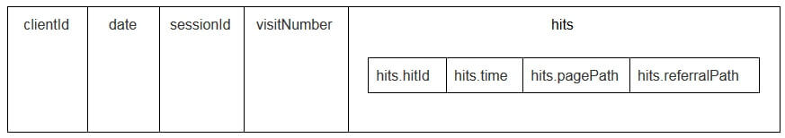
The hits table contains information about user actions on the site. For example, if a user clicks on a banner, flips through the catalog, opens a product page, puts a product in the basket, or places an order, these actions will be recorded in the hits table.

If a user places an order on the site, information about the order will also be entered in the hits table:

transactionId (number identifying the transaction)
transactionRevenue (total value of the order)
transactionShipping (shipping costs)

Session data tables collected using OWOX BI have a similar structure.

Suppose you want to know the number of orders from users in New York City over the past month. To find out, you need to refer to the hits table and count the number of unique transaction IDs. To extract data from such tables, Standard SQL has an UNNEST function:

    
#standardSQL 
SELECT 
COUNT (DISTINCT hits.transaction.transactionId) -- count the number of unique order numbers; DISTINCT helps to avoid duplication
FROM `project_name.dataset_name.owoxbi_sessions_*` -- refer to the table group (wildcard tables)
WHERE 
  (
  _TABLE_SUFFIX BETWEEN FORMAT_DATE('%Y%m%d',DATE_SUB(CURRENT_DATE(),   INTERVAL 1 MONTHS)) -- if we don’t know which dates we need, it’s better to use the function FORMAT_DATE INTERVAL 
  AND
  FORMAT_DATE('%Y%m%d',DATE_SUB(CURRENT_DATE(), INTERVAL 1 DAY)) 
  ) 
AND geoNetwork.city = ‘New York’ -- choose orders made in New York City

If the order information was recorded in a separate table and not in a nested table, you would have to use JOIN to combine the table with order information and the table with session data in order to find out in which sessions orders were made.

More subquery options

If you need to extract data from multi-level nested fields, you can add subqueries with SELECT and WHERE. For example, in OWOX BI session streaming tables, another subtable, product, is written to the hits subtable. The product subtable collects product data that’s transmitted with an Enhanced Ecommerce array. If enhanced e-commerce is set up on the site and a user has looked at a product page, characteristics of this product will be recorded in the product subtable.

To get these product characteristics, you’ll need a subquery inside the main query. For each product characteristic, a separate SELECT subquery is created in parentheses:

    
SELECT 
  column_name1, -- list the other columns you want to receive
  column_name2,
  (SELECT productBrand FROM UNNEST(hits.product)) AS    hits_product_productBrand,
  (SELECT productRevenue FROM UNNEST(hits.product)) AS hits_product_productRevenue, -- list product features
  (SELECT localProductRevenue FROM UNNEST(hits.product)) AS hits_product_localProductRevenue,
  (SELECT productPrice FROM UNNEST(hits.product)) AS hits_product_productPrice,
FROM `project_name.dataset_name.owoxbi_sessions_YYYYMMDD`

Thanks to the capabilities of Standard SQL, it’s easier to build query logic and write code. For comparison, in Legacy SQL, you would need to write this type of ladder:

    
SELECT 
  column_name1,
  column_name2, 
  column_name3 
FROM (
  SELECT table_name.some_column AS column1…
  FROM table_name
)

Requests to external sources

Using Standard SQL, you can access BigQuery tables directly from Google Bigtable, Google Cloud Storage, Google Drive, and Google Sheets.
That is, instead of loading the entire table into BigQuery, you can delete the data with one single query, select the parameters you need, and upload them to cloud storage.

More user functions (UDF)

If you need to use a formula that isn’t documented, User Defined Functions (UDF) will help you. In our practice, this happens rarely, since the Standard SQL documentation covers almost all tasks of digital analytics.

In Standard SQL, user-defined functions can be written in SQL or JavaScript; Legacy SQL only supports JavaScript. The arguments of these functions are columns, and the values they take are the result of manipulating columns. In Standard SQL, functions can be written in the same window as queries.

More JOIN conditions

In Legacy SQL, JOIN conditions can be based on equality or column names. In addition to these options, the Standard SQL dialect supports JOIN by inequality and by arbitrary expression.

For example, to identify unfair CPA partners, we can select sessions in which the source was replaced within 60 seconds of the transaction. To do this in Standard SQL, we can add an inequality to the JOIN condition:

    
#standardSQL
SELECT *
FROM 
  (
  SELECT
  traff.clientId AS clientId,
  traff.page_path AS pagePath,
  traff.traffic_source AS startSource,
  traff.traffic_medium AS startMedium,
  traff.time AS startTime,
  aff.evAction AS evAction,
  aff.evSource AS finishSource,
  aff.evMedium AS finishMedium,
  aff.evCampaign AS finishCampaign,
  aff.time AS finishTime,
  aff.isTransaction AS isTransaction,
  aff.pagePath AS link,
  traff.time-aff.time AS diff
  FROM
    (
    SELECT 
    fullVisitorID AS clientId,
    h.page.pagePath AS page_path,
    trafficSource.source AS traffic_source,
    trafficSource.medium AS traffic_medium,
    trafficSource.campaign AS traffic_campaign,
    date,
    SAFE_CAST(visitStartTime+h.time/1000 AS INT64) AS time
      FROM `demoproject.google_analytics_sample.ga_sessions_20190301`,
      UNNEST (hits) AS h
      WHERE trafficSource.medium != 'cpa'
      ) AS traff
JOIN (
  SELECT 
  total.date date,
  total.time time,
  total.clientId AS clientId,
  total.eventAction AS evAction,
  total.source AS evSource,
  total.medium AS evMedium,
  total.campaign AS evCampaign,
  tr.eventAction AS isTransaction,
  total.page_path AS pagePath
  FROM 
  (
  SELECT 
  fullVisitorID AS clientId,
  h.page.pagePath AS page_path,
  h.eventInfo.eventAction AS eventAction, 
  trafficSource.source AS source,
  trafficSource.medium AS medium,
  trafficSource.campaign AS campaign,
  date,
  SAFE_CAST(visitStartTime+h.time/1000 AS INT64) AS time
  FROM `demoproject.google_analytics_sample.ga_sessions_20190301`,
  UNNEST(hits) AS h
    WHERE
    trafficSource.medium ='cpa'
    ) AS total
LEFT JOIN 
  (
  SELECT
  fullVisitorID AS clientId,
  date,
  h.eventInfo.eventAction AS eventAction,
  h.page.pagePath pagePath,
  SAFE_CAST(visitStartTime+h.time/1000 AS INT64) AS time
  FROM `demoproject.google_analytics_sample.ga_sessions_20190301`,
  UNNEST(hits) AS h
  WHERE h.eventInfo.eventAction = 'typ_page'
  AND h.type = 'EVENT'
  GROUP BY 1, 2, 3, 4, 5
  ) AS tr
ON total.clientId=tr.clientId
AND total.date=tr.date
AND tr.time>total.time -- JOIN tables by inequality. Pass the additional WHERE clause that was needed in Legacy SQL
WHERE tr.eventAction = 'typ_page'
  ) AS aff
ON traff.clientId = aff.clientId
)
WHERE diff> -60
AND diff<0
  GROUP BY 1, 2, 3, 4, 5, 6, 7, 8, 9, 10, 11, 12, 13
  ORDER BY clientId, finishTime

The only limitation of Standard SQL with respect to JOIN is that it doesn’t allow semi-join with subqueries of the form WHERE column IN (SELECT ...):

    
#legacySQL
SELECT
  mother_age,
  COUNT(mother_age) total
FROM
  [bigquery-public-data:samples.natality]
WHERE -- such a construction cannot be used in Standard SQL
  state IN (SELECT
              state
            FROM
              (SELECT
                 state,
                 COUNT(state) total
               FROM
                 [bigquery-public-data:samples.natality]
               GROUP BY
                 state
               ORDER BY
                 total DESC
               LIMIT 10))
  AND mother_age > 50
GROUP BY
  mother_age
ORDER BY
  mother_age DESC

Less chance of mistakes

Some functions in Legacy SQL return NULL if the condition is incorrect. For example, if division by zero has crept into your calculations, the query will be executed and NULL entries will appear in the resulting rows of the table. This may mask problems in the query or in the data.

The logic of Standard SQL is more straightforward. If a condition or input data is incorrect, the query will generate an error, for example «division by zero,» so you can quickly correct the query. The following checks are embedded in Standard SQL:

Valid values for +, -, ×, SUM, AVG, STDEV
Division by zero

Requests run faster

JOIN queries written in Standard SQL are faster than those written in Legacy SQL thanks to preliminary filtering of incoming data. First, the query selects the rows that match the JOIN conditions, then processes them.

In the future, Google BigQuery will work on improving the speed and performance of queries only for Standard SQL.

Tables can be edited: insert and delete rows, update

Data Manipulation Language (DML) functions are available in Standard SQL. This means that you can update tables and add or remove rows from them through the same window in which you write queries. For example, using DML, you can combine data from two tables into one:

    
#standardSQL
MERGE dataset.Inventory AS T
USING dataset.NewArrivals AS S
ON T.ProductID = S.ProductID
WHEN MATCHED THEN
  UPDATE SET quantity = T.quantity + S.quantity
WHEN NOT MATCHED THEN
  INSERT (ProductID, quantity) VALUES (ProductID, quantity)

Code is easier to read and edit

With Standard SQL, complex queries can be started not only with SELECT but also with WITH, making code easier to read, comment, and understand. This also means it’s easier to prevent your own and correct others’ mistakes.

    
#standardSQL
WITH total_1 AS ( -- the first subquery in which the intermediate indicator will be calculated
    SELECT
        id,
        metric1,
       SUM(metric2) AS total_sum1
    FROM `project_name.dataset_name.owoxbi_sessions_YYYYMMDD`
    GROUP BY
        id, metric
),
total_2 AS ( -- the second subquery
    SELECT
        id,
        metric1,
        SUM(metric2) AS total_sum2
    FROM `project_name.dataset_name.owoxbi_sessions_YYYYMMDD`
           GROUP BY
        id, metric1
),
total_3 AS ( -- the third subquery
    SELECT
        id,
        metric,
       SUM(metric2) AS total_sum3
       FROM `project_name.dataset_name.owoxbi_sessions_YYYYMMDD`
    GROUP BY
        id, metric
)
SELECT *,
ROUND(100*( total_2.total_sum2 - total_3.total_sum3) / total_3.total_sum3, 3) AS difference -- get the difference index: subtract the value of the second subquery from the value of the third; divide by the value of the third 
FROM total_1
ORDER  BY 1, 2

It’s convenient to work with the WITH operator if you have calculations that are done in several stages. First, you can collect intermediate metrics in subqueries, then do the final calculations.

The Google Cloud Platform (GCP), which includes BigQuery, is a full-cycle platform for working with big data, from organizing a data warehouse or data cloud to running scientific experiments and predictive and prescriptive analytics. With the introduction of Standard SQL, BigQuery is expanding its audience. Working with GCP is becoming more interesting for marketing analysts, product analysts, data scientists, and teams of other specialists.

Capabilities of Standard SQL and examples of use cases

At OWOX BI, we often work with tables compiled using the standard Google Analytics 360 export to Google BigQuery or the OWOX BI Pipeline. In the examples below, we’ll look at the specifics of SQL queries for such data.

If you aren’t already collecting data from your site in BigQuery, you can try doing so for free with the trial version of OWOX BI.

BOOK A DEMO

1. Select data for a time interval

In Google BigQuery, user behavior data for your site is stored in wildcard tables (tables with an asterisk); a separate table is formed for each day. These tables have the same name: only the suffix is different. The suffix is the date in the format YYYYMMDD. For example, the table owoxbi_sessions_20190301 contains data on sessions for March 1, 2019.

We can refer directly to a group of such tables in one request in order to obtain data, for example, from February 1 through February 28, 2019. To do this, we need to replace YYYYMMDD with an * in FROM, and in WHERE, we need to specify the table suffixes for the start and end of the time interval:

    
#standardSQL
SELECT sessionId, 
FROM `project_name.dataset_name.owoxbi_sessions_*`
WHERE _TABLE_SUFFIX BETWEEN `20190201` AND `20190228`

The specific dates for which we want to collect data are not always known to us. For example, every week we might need to analyze data for the last three months. To do this, we can use the FORMAT_DATE function:

    
#standardSQL
SELECT
 <enumerate field names>
FROM `project_name.dataset_name.owoxbi_sessions_*`
WHERE 
_TABLE_SUFFIX BETWEEN FORMAT_DATE('%Y%m%d',DATE_SUB(CURRENT_DATE(), INTERVAL 3 MONTHS))
AND
FORMAT_DATE('%Y%m%d',DATE_SUB(CURRENT_DATE(), INTERVAL 1 DAY))

After BETWEEN, we record the suffix of the first table. The phrase CURRENT_DATE (), INTERVAL 3 MONTHS means «select data for the last 3 months from the current date.» The second table suffix is formatted after AND. It’s needed to mark the end of the interval as yesterday: CURRENT_DATE (), INTERVAL 1 DAY.

2. Retrieve user parameters and indicators

User parameters and metrics in Google Analytics Export tables are written to the nested hits table and to the customDimensions and customMetrics subtables. All custom dimensions are recorded in two columns: one for the number of parameters collected on the site, the second for their values. Here’s what all the parameters transmitted with one hit look like:

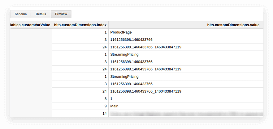
In order to unpack them and write the necessary parameters in separate columns, we use the following SQL query:

    
-- Custom Dimensions (in the line below index - the number of the user variable, which is set in the Google Analytics interface; dimension1 is the name of the custom parameter, which you can change as you like. For each subsequent parameter, you need to write the same line:

  (SELECT MAX(IF(index=1, value, NULL)) FROM UNNEST(hits.customDimensions)) AS dimension1, 
-- Custom Metrics: the index below is the number of the user metric specified in the Google Analytics interface; metric1 is the name of the metric, which you can change as you like. For each of the following metrics, you need to write the same line: 

  (SELECT MAX(IF(index=1, value, NULL)) FROM UNNEST(hits.customMetrics)) AS metric1

Here’s what it looks like in the request:

    
#standardSQL
SELECT <column name1>,
<column_name2>, -- list column names
(SELECT MAX(IF(index=1, value, NULL)) FROM UNNEST(hits.customDimensions)) AS page_type,
(SELECT MAX(IF(index=2, value, NULL)) FROM UNNEST(hits.customDimensions)) AS visitor_type, -- produce the necessary custom dimensions
(SELECT MAX(IF(index=1, value, NULL)) FROM UNNEST(hits.customMetrics)) AS metric1 -- produce the necessary custom metrics
<column_name3> -- if you need more columns, continue to list
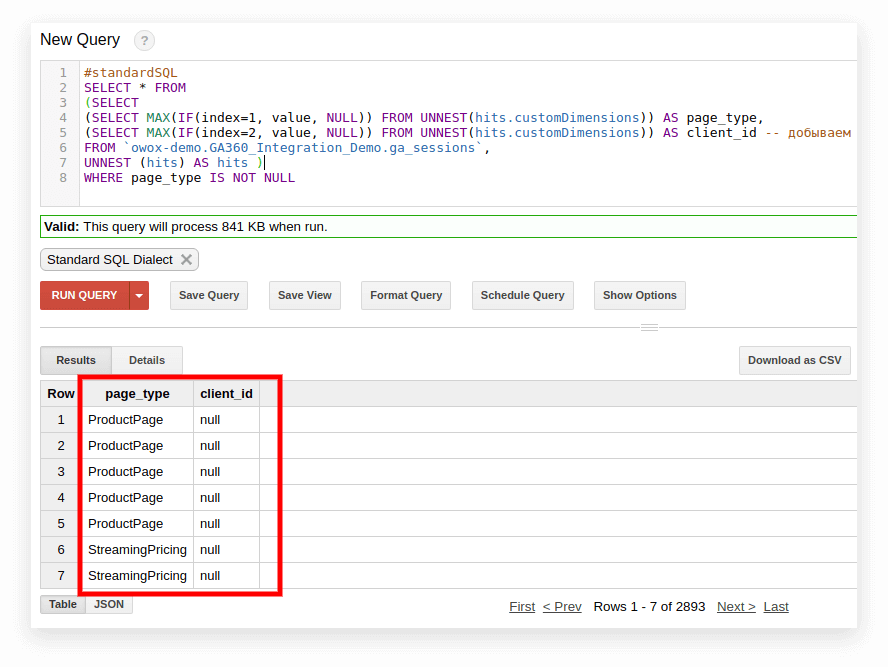
FROM `project_name.dataset_name.owoxbi_sessions_20190201`

In the screenshot below, we’ve selected parameters 1 and 2 from Google Analytics 360 demo data in Google BigQuery and called them page_type and client_id. Each parameter is recorded in a separate column:

3. Calculate the number of sessions by traffic source, channel, campaign, city, and device category

Such calculations are useful if you plan to visualize data in Google Data Studio and filter by city and device category. This is easy to do with the COUNT window function:

    
#standardSQL
SELECT
<column_name 1>, -- choose any columns 
COUNT (DISTINCT sessionId) AS total_sessions, -- summarize the session IDs to find the total number of sessions
COUNT(DISTINCT sessionId) OVER(PARTITION BY date, geoNetwork.city, session.device.deviceCategory, trafficSource.source, trafficSource.medium, trafficSource.campaign) AS part_sessions -- summarize the number of sessions by campaign, channel, traffic source, city, and device category
FROM `project_name.dataset_name.owoxbi_sessions_20190201`

4. Merge the same data from several tables

Suppose you collect data on completed orders in several BigQuery tables: one collects all orders from Store A, the other collects orders from Store B. You want to combine them into one table with these columns:

client_id — a number that identifies a unique buyer
transaction_created — order creation time in TIMESTAMP format
transaction_id — order number
is_approved — whether the order was confirmed
transaction_revenue — order amount

In our example orders from January 1, 2018, to yesterday must be in the table. To do this, select the appropriate columns from each group of tables, assign them the same name, and combine the results with UNION ALL:

    
#standardSQL
SELECT 
cid AS client_id, 
order_time AS transaction_created,
order_status AS is_approved,
order_number AS transaction_id
FROM `project_name.dataset_name.table1_*`
WHERE (
  _TABLE_SUFFIX BETWEEN `20180101`
  AND
  FORMAT_DATE('%Y%m%d',DATE_SUB(CURRENT_DATE(), INTERVAL 1 DAY))
  )

UNION ALL 
SELECT
userId AS client_id,
created_timestamp AS transaction_created,
operator_mark AS  is_approved,
transactionId AS transaction_id
FROM `project_name.dataset_name.table1_*`
WHERE (
  _TABLE_SUFFIX BETWEEN `20180101`
  AND
  FORMAT_DATE('%Y%m%d',DATE_SUB(CURRENT_DATE(), INTERVAL 1 DAY))
  )
ORDER BY transaction_created DESC

5. Create a dictionary of traffic channel groups

When data enters Google Analytics, the system automatically determines the group to which a particular transition belongs: Direct, Organic Search, Paid Search, and so on. To identify a group of channels, Google Analytics looks at the UTM tags of transitions, namely utm_source and utm_medium. You can read more about channel groups and definition rules in Google Analytics Help.

If OWOX BI clients want to assign their own names to groups of channels, we create a dictionary, which transition belongs to a specific channel. To do this, we use the conditional CASE operator and the REGEXP_CONTAINS function. This function selects the values in which the specified regular expression occurs.

We recommend taking names from your list of sources in Google Analytics. Here’s an example of how to add such conditions to the request body:

    
#standardSQL
SELECT 
CASE 
WHEN (REGEXP_CONTAINS (source, 'google') AND medium = 'referral' THEN 'Organic Search' 
WHEN (REGEXP_CONTAINS (source, 'yahoo')) AND medium = 'referral' THEN 'Referral'
WHEN (REGEXP_CONTAINS (source, '^(go.mail.ru|google.com)$') AND medium = 'referral') THEN 'Organic Search'
WHEN medium = 'organic' THEN 'Organic Search'
WHEN (medium = 'cpc') THEN 'Paid Search'
WHEN REGEXP_CONTAINS (medium, '^(sending|email|mail)$') THEN 'Email'
    WHEN REGEXP_CONTAINS (source, '(mail|email|Mail)') THEN 'Email'
    WHEN REGEXP_CONTAINS (medium, '^(cpa)$') THEN 'Affiliate'
    WHEN medium = 'social' THEN 'Social'
    WHEN source = '(direct)' THEN 'Direct'
 WHEN REGEXP_CONTAINS (medium, 'banner|cpm') THEN 'Display'
    ELSE 'Other'
  END channel_group -- the name of the column in which the channel groups are written
FROM `project_name.dataset_name.owoxbi_sessions_20190201`

How to switch to Standard SQL

If you haven’t switched to Standard SQL yet, you can do it at any time. The main thing is to avoid mixing dialects in one request.

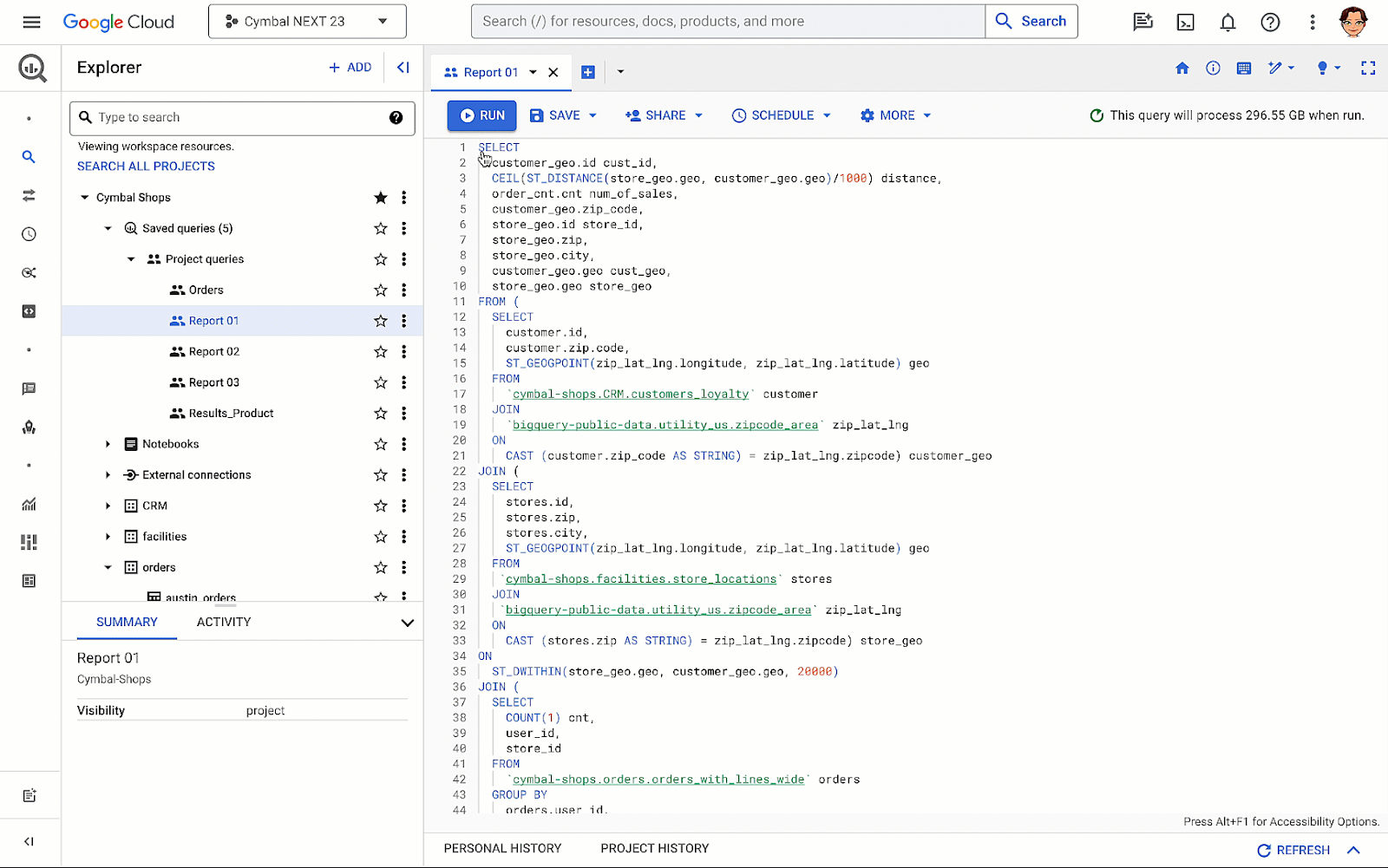
Option 1. Switch in the Google BigQuery interface

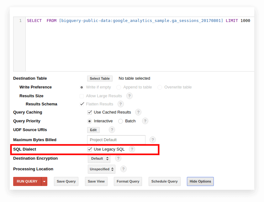
Legacy SQL is used by default in the old BigQuery interface. To switch between dialects, click Show Options under the query input field and uncheck the Use Legacy SQL box next to SQL Dialect.

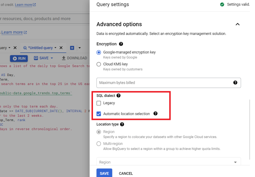
The new interface uses Standard SQL by default. Here, you need to go to the More tab to switch dialects:

Option 2. Write the prefix at the beginning of the request

If you haven’t ticked the request settings, you can start with the desired prefix (#standardSQL or #legacySQL):

    
#standardSQL
SELECT
  weight_pounds, state, year, gestation_weeks
FROM
  `bigquery-public-data.samples.natality`
ORDER BY weight_pounds DESC
LIMIT 10;

In this case, Google BigQuery will ignore the settings in the interface and run the query using the dialect specified in the prefix.

If you have views or saved queries that are launched on a schedule using Apps Script, don’t forget to change the value of useLegacySql to false in the script:

    
var job = {
configuration: {
  query: {
    query: 'INSERT INTO MyDataSet.MyFooBarTable (Id, Foo, Date) VALUES (1, \'bar\', current_Date);',
    useLegacySql: false
    }

Option 3. Transition to Standard SQL for views

If you work with Google BigQuery not with tables but with views, those views can’t be accessed in the Standard SQL dialect. That is, if your presentation is written in Legacy SQL, you can’t write requests to it in Standard SQL.

To transfer a view to standard SQL, you need to manually rewrite the query by which it was created. The easiest way to do this is through the BigQuery interface.

1. Open the view:

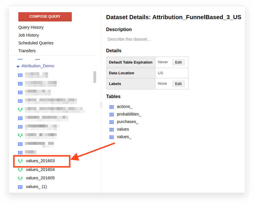
2. Click Details. The query text should open, and the Edit Query button will appear below:

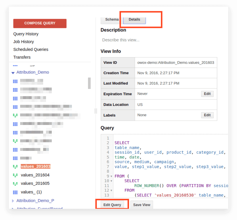
Now you can edit the request according to the rules of Standard SQL.
If you plan to continue using the request as a presentation, click Save View after you’ve finished editing.

Compatibility, syntax features, operators, functions

Compatibility

Thanks to the implementation of Standard SQL, you can directly access data stored in other services directly from BigQuery:

Google Cloud Storage log files
Transactional records in Google Bigtable
Data from other sources

This allows you to use Google Cloud Platform products for any analytical tasks, including predictive and prescriptive analytics based on machine learning algorithms.

Query syntax

The query structure in the Standard dialect is almost the same as in Legacy:

WITH <request alias> AS <expression>

SELECT <fields or expressions you want to get in result>

FROM <the name of a table or a view>,

UNNEST <the name of the nested field, if your query contains calls to nested fields> AS <nested field alias>

WHERE <conditions for result filter>

GROUP BY <columns to group the result>

HAVING <a condition similar to WHERE for aggregation functions>

JOIN <the name of a table or view #2> ON <conditions> | USING <the name of the columns to merge tables>

ORDER BY <by which columns to sort the result> DESC | ASC

LIMIT <how many lines to output> OFFSET <how many lines to skip from the start>

The names of the tables and view are separated with a period (full stop), and the whole query is enclosed in grave accents: `project_name.data_name_name.table_name`.

For example `bigquery-public-data.samples.natality`.

The full syntax of the query, with explanations of what can be included in each operator, is compiled as a schema in the BigQuery documentation.

Features of Standard SQL syntax:

Commas are needed to list fields in the SELECT statement.
If you use the UNNEST operator after FROM , a comma or JOIN is placed before UNNEST.
You can’t put a comma before FROM.
A comma between two queries equals a CROSS JOIN, so be careful with it.
JOIN can be done not only by column or equality but by arbitrary expressions and inequality.
It’s possible to write complex subqueries in any part of the SQL expression (in SELECT, FROM, WHERE, etc.). In practice, it’s not yet possible to use expressions like WHERE column_name IN (SELECT ...) as you can in other databases.

Operators

In Standard SQL, operators define the type of data. For example, an array is always written in brackets []. Operators are used for comparison, matching the logical expression (NOT, OR, AND), and in arithmetic calculations.

Functions

Standard SQL supports more features than Legacy: traditional aggregation (sum, number, minimum, maximum); mathematical, string, and statistical functions; and rare formats such as HyperLogLog ++.

In the Standard dialect, there are more functions for working with dates and TIMESTAMP. A complete list of features is provided in Google’s documentation. The most commonly used functions are for working with dates, strings, aggregation, and window.

1. Aggregation functions

COUNT (DISTINCT column_name) counts the number of unique values in a column. For example, say we need to count the number of sessions from mobile devices on March 1, 2019. Since a session number can be repeated on different lines, we want to count only the unique session number values:

    
#standardSQL
SELECT 
COUNT (DISTINCT sessionId) AS sessions
FROM  `project_name.dataset_name.owoxbi_sessions_20190301`
WHERE device.deviceCategory = 'mobile'

SUM (column_name) — the sum of the values in the column

    
#standardSQL
SELECT 
SUM (hits.transaction.transactionRevenue) AS revenue
FROM  `project_name.dataset_name.owoxbi_sessions_20190301`,
UNNEST (hits) AS hits -- unpacking the nested field hits
WHERE device.deviceCategory = 'mobile'

MIN (column_name) | MAX (column_name) — the minimum and maximum value in the column. These functions are convenient for checking the spread of data in a table.

2. Window (analytical) functions

Analytical functions consider values not for the entire table but for a certain window — a set of rows that you’re interested in. That is, you can define segments within a table. For example, you can calculate SUM (revenue) not for all lines but for cities, device categories, and so on. You can turn the analytic functions SUM, COUNT, and AVG as well as other aggregation functions by adding the OVER condition (PARTITION BY column_name) to them.

For example, you need to count the number of sessions by traffic source, channel, campaign, city, and device category. In this case, we can use the following expression:

    
SELECT
        date,
        geoNetwork.city,
        t.device.deviceCategory,
        trafficSource.source,
        trafficSource.medium,
        trafficSource.campaign,
COUNT(DISTINCT sessionId) OVER(PARTITION BY date, geoNetwork.city, session.device.deviceCategory, trafficSource.source, trafficSource.medium, trafficSource.campaign) AS segmented_sessions
FROM  `project_name.dataset_name.owoxbi_sessions_20190301` t

OVER determines the window for which calculations will be made. PARTITION BY indicates which rows should be grouped for calculation. In some functions, it’s necessary to specify the order of grouping with ORDER BY.

For a complete list of window functions, see the BigQuery documentation.

3. String functions

These are useful when you need to change text, format the text in a line, or glue the values of columns. For example, string functions are great if you want to generate a unique session identifier from the standard Google Analytics 360 export data. Let’s consider the most popular string functions.

SUBSTR cuts part of the string. In the request, this function is written as SUBSTR (string_name, 0.4). The first number indicates how many characters to skip from the beginning of the line, and the second number indicates how many digits to cut. For example, say you have a date column that contains dates in the STRING format. In this case, the dates look like this: 20190103. If you want to extract a year from this line, SUBSTR will help you:

    
#standardSQL
SELECT
SUBSTR(date,0,4) AS year
FROM `project_name.dataset_name.owoxbi_sessions_20190301`

CONCAT (column_name, etc.) glues values. Let’s use the date column from the previous example. Suppose you want all dates to be recorded like this: 2019-03-01. To convert dates from their current format to this format, two string functions can be used: first, cut the necessary pieces of the string with SUBSTR, then glue them through the hyphen:

    
#standardSQL
SELECT
CONCAT(SUBSTR(date,0,4),"-",SUBSTR(date,5,2),"-",SUBSTR(date,7,2)) AS date
FROM `project_name.dataset_name.owoxbi_sessions_20190301`

REGEXP_CONTAINS returns the values of columns in which the regular expression occurs:

    
#standardSQL
SELECT 
CASE
WHEN REGEXP_CONTAINS (medium, '^(sending|email|mail)$') THEN 'Email'
    WHEN REGEXP_CONTAINS (source, '(mail|email|Mail)') THEN 'Email'
    WHEN REGEXP_CONTAINS (medium, '^(cpa)$') THEN 'Affiliate'
ELSE 'Other'
END Channel_groups
FROM `project_name.dataset_name.owoxbi_sessions_20190301`

This function can be used in both SELECT and WHERE. For example, in WHERE, you can select specific pages with it:

    
WHERE REGEXP_CONTAINS(hits.page.pagePath, 'land[123]/|/product-order')

4. Date functions

Often, dates in tables are recorded in STRING format. If you plan to visualize results in Google Data Studio, the dates in the table need to be converted to DATE format using the PARSE_DATE function.

PARSE_DATE converts a STRING of the 1900-01-01 format to the DATE format.

If the dates in your tables look different (for example, 19000101 or 01_01_1900), you must first convert them to the specified format.

    
#standardSQL
SELECT 
PARSE_DATE('%Y-%m-%d', date)  AS date_new
FROM `project_name.dataset_name.owoxbi_sessions_20190301`

DATE_DIFF calculates how much time has passed between two dates in days, weeks, months, or years. It’s useful if you need to determine the interval between when a user saw advertising and placed an order. Here’s how the function looks in a request:

    
#standardSQL 
SELECT DATE_DIFF( 
PARSE_DATE('%Y%m%d', date1), PARSE_DATE('%Y%m%d', date2), DAY 
) days -- convert the date1 and date2 lines to the DATE format; choose units to show the difference (DAY, WEEK, MONTH, etc.)
FROM `project_name.dataset_name.owoxbi_sessions_20190301`

If you want to learn more about the listed functions, read BigQuery Google Features — A Detailed Review.

SQL queries for marketing reports

The Standard SQL dialect allows businesses to extract maximum information from data with deep segmentation, technical audits, marketing KPI analysis, and identification of unfair contractors in CPA networks. Here are examples of business problems in which SQL queries on data collected in Google BigQuery will help you.

1. ROPO analysis: evaluate the contribution of online campaigns to offline sales. To perform ROPO analysis, you need to combine data on online user behavior with data from your CRM, call tracking system, and mobile application.

If there’s a key in one and the second base — a common parameter that is unique for each user (for example, User ID) — you can track:

which users visited the site before buying goods in the store
how users behaved on the site
how long users took to make a purchase decision
what campaigns had the greatest increase on offline purchases.

2. Segment customers by any combination of parameters, from behavior on the site (pages visited, products viewed, number of visits to the site before buying) to loyalty card number and purchased items.

3. Find out which CPA partners are working in bad faith and replacing UTM tags.

4. Analyze the progress of users through the sales funnel.

We’ve prepared a selection of queries in Standard SQL dialect. If you already collect data from your site, from advertising sources, and from your CRM system in Google BigQuery, you can use these templates to solve your business problems. Simply replace the project name, dataset, and table in BigQuery with your own. In the collection, you’ll receive 11 SQL queries.

For data collected using standard export from Google Analytics 360 to Google BigQuery:

User actions in the context of any parameters
Statistics on key user actions
Users who viewed specific product pages
Actions of users who bought a particular product
Set up the funnel with any necessary steps
Effectiveness of the internal search site

For data collected in Google BigQuery using OWOX BI:

Attributed consumption by source and channel
Average cost of attracting a visitor by city
ROAS for gross profit by source and channel
Number of orders in the CRM by payment method and delivery method
Average delivery time by city

bonus for readers

SQL templates for Google Analytics 360 and Google Analytics 4 schemas

Download now

If you have questions about querying Google BigQuery data that you didn’t find answers to in this article, ask in the comments. We’ll try to help you.