7 Google Sheets features every marketer should know
Seven Google Sheets features cover most of what a marketing report needs: pivot tables to summarize campaigns, conditional formatting to flag what is off, charts to show trends, dropdowns to keep channel names consistent, filters to focus on a segment, QUERY to build summaries with one formula, and IMPORTRANGE to combine spreadsheets. Each comes with an example and a link to the full guide.
Most marketing reports in Google Sheets are built from the same seven features. Each one below has a short example and a link to its full guide.
| Feature | What a marketer uses it for |
|---|---|
| 1. Pivot tables | Spend, clicks and conversions by channel, campaign or week |
| 2. Conditional formatting | Flag campaigns above a cost limit or below a target |
| 3. Charts and sparklines | Trends over time, comparison of channels |
| 4. Dropdowns and data validation | One spelling for every channel and status |
| 5. Filters and slicers | A look at one channel, region or period |
| 6. QUERY | A summary table from one formula |
| 7. IMPORTRANGE | Data from other spreadsheets in one report |
1. Pivot tables: summarize campaigns in a minute
1. Pivot tables: summarize campaigns in a minute
A pivot table groups rows and totals them without a single formula. Select the data, choose Insert > Pivot table, put the dimension into Rows and the metrics into Values.
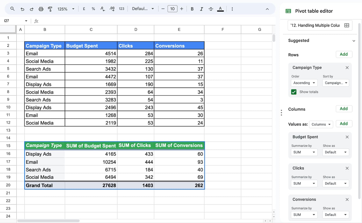
In the screenshot, the campaign rows become four lines, one per campaign type. The totals are where the analysis starts: Display Ads spent 4,165 for 60 conversions, about 69 per conversion, while Search Ads spent 6,715 for 40, about 168. A calculated field in the pivot table, spend divided by conversions, puts that ratio next to the totals.
Full guide: pivot tables, and pivot charts for charting the result.
2. Conditional formatting: see what needs attention
2. Conditional formatting: see what needs attention
Conditional formatting colors the cells that meet a rule: a cost per lead above the limit, a conversion rate below the target, a budget that is nearly spent. Select the range, choose Format > Conditional formatting, and set the rule.
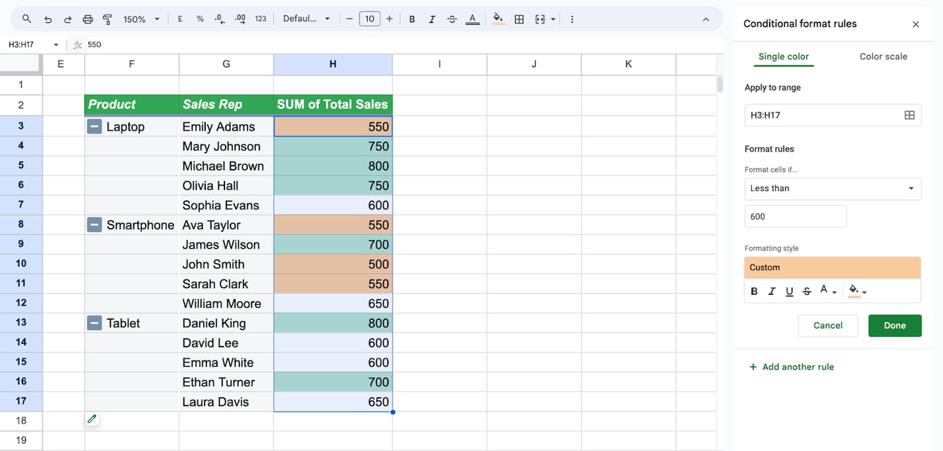
Two rules cover most reports:
- A threshold. “Greater than” or “Less than” a number, as in the screenshot.
- A color scale. A gradient from the lowest to the highest value, which turns a column of numbers into a heat map.
With Custom formula is, a rule can color a whole row based on one column: =$E3 > 100 applied to B3:F20 colors every row where column E exceeds 100.
OWOX Data Marts
See your first report built in real time. 15 minutes.
- Connect your data warehouse
- Pick your metrics
- Get a live Google Sheets report
In the time it takes to write a ticket. Then imagine never writing that ticket again.
Book a DemoWe'll use your actual use case
3. Charts: show the trend, not the table
3. Charts: show the trend, not the table
A line chart for a metric over time, a column or bar chart for channels side by side. Select the data and choose Insert > Chart; the type is changed in the editor.
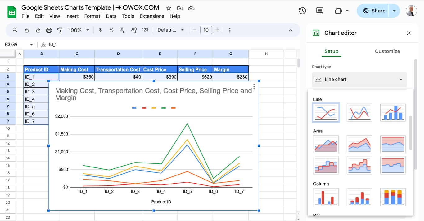
For a trend inside a single cell, next to each campaign in a table, use SPARKLINE.
Full guides: charts for visualization, bar graphs, pivots and charts.
4. Dropdowns and data validation: one name per channel
4. Dropdowns and data validation: one name per channel
“Facebook”, “facebook” and “FB” are three channels to a pivot table. A dropdown makes them one. Select the column, choose Data > Data validation, add a rule with Dropdown and list the allowed values; anything else is rejected or marked.
This matters most in the sheets people fill by hand: campaign plans, budgets, UTM builders, content calendars. Full guide: data validation. When the mess is already there, find and replace and TRIM clean it up.
5. Filters and slicers: one segment at a time
5. Filters and slicers: one segment at a time
Data > Create a filter adds a menu to each header for sorting and for hiding rows. A filter view does the same for you alone, without changing what colleagues see. A slicer is a filter control placed on the sheet, for charts and pivot tables in a dashboard.
The FILTER function returns the matching rows as a formula, in another place, and stays up to date:
=FILTER(B3:E17, C3:C17="Financial Software")
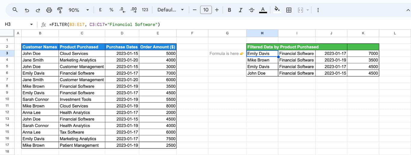
Full guides: FILTER, how to sort data.
6. QUERY: a summary from one formula
6. QUERY: a summary from one formula
QUERY filters, groups and sorts a range with a short SQL-like text. The simplest form returns the rows that meet a condition:
=QUERY(B2:D17, "SELECT * WHERE B = 'John Smith'")
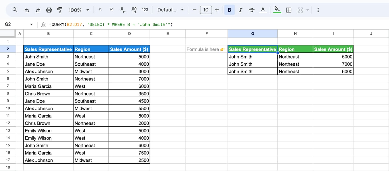
Its strength is the summary. With channels in column B, spend in C and conversions in D, one formula returns spend and conversions per channel, largest spend first:
=QUERY(B2:D100, "SELECT B, SUM(C), SUM(D) GROUP BY B ORDER BY SUM(C) DESC", 1)
Unlike a pivot table, the result is a formula: it can sit inside a report layout and feed other formulas. Full guides: QUERY, date filtering with QUERY.
7. IMPORTRANGE: one report from several spreadsheets
7. IMPORTRANGE: one report from several spreadsheets
IMPORTRANGE reads a range from another spreadsheet, for example the budget file of the finance team or the plan of each regional team:
=IMPORTRANGE("spreadsheet URL", "Finance2024!B2:D14")
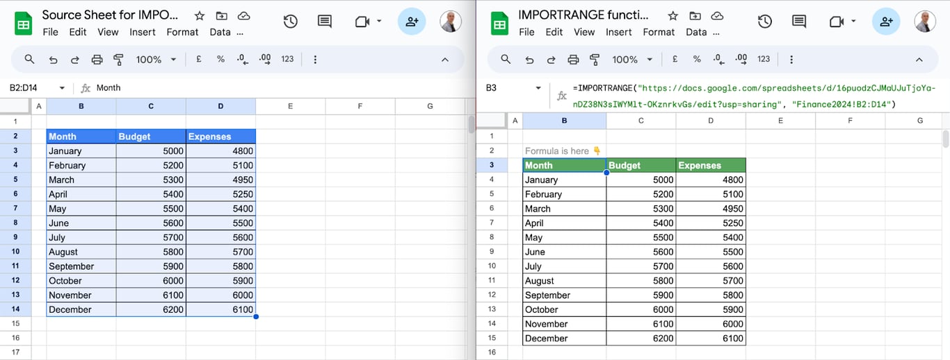
The first time two files are connected, the formula asks for access to the source file. After that the data follows the source. Combined with QUERY, it imports only the rows and columns the report needs.
Full guides: IMPORTRANGE, QUERY with IMPORTRANGE, linking data across sheets.
The formulas behind marketing metrics
The formulas behind marketing metrics
The features above arrange the data. The metrics themselves are simple divisions, wrapped in IFERROR so that a campaign with zero clicks does not show an error:
| Metric | Formula |
|---|---|
| Click-through rate | =IFERROR(clicks / impressions, 0) |
| Cost per click | =IFERROR(spend / clicks, 0) |
| Conversion rate | =IFERROR(conversions / clicks, 0) |
| Cost per conversion | =IFERROR(spend / conversions, 0) |
| Return on ad spend | =IFERROR(revenue / spend, 0) |
Calculate a ratio for a group from the totals, total spend divided by total conversions, not as an average of the row ratios.
Functions worth knowing next:
- SUMIF and SUMIFS: Spend or revenue by channel and period.
- COUNTIF and COUNTIFS: Leads or orders by condition.
- VLOOKUP and XLOOKUP: Add a campaign’s owner, budget or category from another table.
- REGEX functions: Take the source or campaign out of a UTM-tagged URL.
- Date functions and WEEKNUM: Group by week and month.
- ARRAYFORMULA: One formula for a whole column.
- GOOGLEFINANCE: Convert spend in several currencies to one.
- UNIQUE: The list of campaigns or channels without repeats.
The features are free; the hours go into getting the data in
The features are free; the hours go into getting the data in
All seven features work on data that is already in the sheet. For a marketer that is the expensive part: exports from each ad platform, pasted every week, in layouts that do not match, with numbers that are a few days old by the time the report is read.
The OWOX Data Marts extension for Google Sheets covers that half. A data analyst publishes a data mart (a table or an SQL query in your data warehouse) and makes it available for reports. In Sheets you open the extension, pick the data mart, tick the columns you want and run it. The rows land in a tab, ready for your formulas.
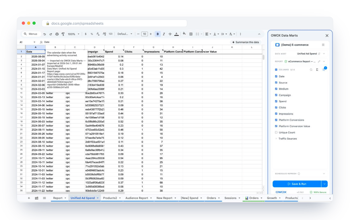
What changes for the person who maintains the sheet:
- Refresh replaces re-export. Refresh current report in the extension menu re-runs the same pull, and a scheduled refresh keeps the tab current without anyone touching it.
- The source is written on the sheet. The header cell of an imported tab carries a note with the data mart it came from, the time of the import and a link to the report.
- No SQL and no warehouse access needed. The analyst decides which data marts and columns are available. You choose from that list.
The extension does not write or change the analyst’s SQL. Pivot tables, charts and QUERY then run on current numbers, and the weekly round of exports is no longer needed for them. The extension comes with the OWOX Cloud plans of OWOX Data Marts; spreadsheet reporting describes both ways data reaches a sheet.
Turn your data into decisions.
Governed data marts give you the clean foundation ML needs to actually work.
- No AI hallucinations
- Analyst-governed definitions
- Every number traces to SQL
Frequently Asked Questions
What role does data validation play in Google Sheets?
Data validation ensures consistency and accuracy by restricting input to predefined criteria, such as dropdown lists or specific ranges. This prevents errors, standardizes data entry, and supports reliable marketing analysis and reporting.
How do charts and graphs enhance marketing reports?
Charts and graphs transform raw data into clear, visual insights, making presenting and interpreting campaign performance easier. They help marketers track trends, compare metrics, and communicate results effectively to stakeholders, ensuring impactful decision-making.
Why are pivot tables important for marketers?
Pivot tables allow marketers to organize and summarize large datasets effortlessly. They help identify trends, segment audiences, and track key performance metrics. Customizable and interactive, pivot tables enable quick insights, making them crucial for data-driven marketing strategies.
Can Google Sheets be used for advanced data analysis?
Yes, Google Sheets supports advanced data analysis with functions like QUERY, IMPORTRANGE, and FILTER. These tools allow marketers to sort, filter, and combine data dynamically, perform complex calculations, and derive actionable insights.
How can conditional formatting help in marketing analysis?
Conditional formatting highlights key data points, such as high-performing campaigns or underperforming metrics, using color-coded rules. This visual representation simplifies data analysis, enabling marketers to spot patterns, monitor KPIs, and address issues effectively.
What are the most useful Google Sheets features for marketers?
Pivot tables, conditional formatting, charts, dropdowns with data validation, filters and slicers, QUERY and IMPORTRANGE. Together they cover summarizing campaigns, flagging what is off target, showing trends, keeping names consistent and combining data from several spreadsheets.